Ansys HPC Case Study: Accelerating a 120-Million Cell Simulation Using MR CFD’s Ansys HPC Service

In the high-stakes world of aerodynamics, fidelity is everything. But as engineers, we often hit a brutal wall: the trade-off between mesh resolution and solve time. Recently, we worked with a client facing this exact dilemma—a massive external aerodynamics project that was literally unsolveable on standard hardware.

This article details how we utilized the ansys hpc pack architecture to transform a project that was stuck in “pending” for weeks into a job completed in mere hours. We will strip away the marketing fluff and look at the raw engineering data: the domain decomposition strategies, the hardware specifications, and the core scaling benchmark results that prove why high-fidelity CFD belongs on the cloud.

---

What Was the Engineering Challenge Facing the Client in large scale cfd simulations?

The client, an emerging R&D group in the automotive sector, was attempting to validate a new side-mirror design for aero-acoustic noise reduction. To capture the turbulent flow structures accurately, they utilized a Detached Eddy Simulation (DES) turbulence model.

The requirements were punishing:

• Mesh Count: 120 Million Cells (Unstructured Poly-Hexcore).
• Physics: Transient, Compressible Flow, DES.
• Time Steps: 20,000 steps required for statistical convergence.

They attempted to run this large-scale aerodynamic simulation on their in-house “high-end” workstation—a dual-socket machine with 32 cores and 128GB of RAM.

The result was a disaster.

The simulation required approximately 180GB of RAM just to load the mesh and initialize. Because their workstation only had 128GB, the operating system began “swapping” to the hard drive (paging). The CPU utilization plummeted to 5%, and the time per iteration skyrocketed to over 45 minutes. At that rate, the simulation would have taken 1.7 years to complete. They were missing deadlines, and their design cycle had ground to a halt.

---

Why Is “Ansys HPC” Architecture Critical for Large Meshes?

There is a fundamental misconception that adding more cores always equals more speed. However, in CFD, memory bandwidth is often the true bottleneck.

When you run a 120-million cell model, the CPU cores need to constantly fetch pressure and velocity data from the RAM. On a standard workstation, even a powerful one, all 32 cores are fighting over a limited number of memory channels. It’s like trying to drain a swimming pool through a drinking straw.

To solve this, you need a true what is hpc architecture.

In a HPC cluster for CFD, we distribute the mesh across multiple physical “nodes” (servers). Each node has its own dedicated memory banks. Instead of 32 cores fighting for 128GB of RAM, we might use 8 nodes, giving us 512 cores and 2 Terabytes of aggregate RAM bandwidth. The critical component that ties this all together is the interconnect—the network cables connecting the servers. Standard Ethernet is too slow; we utilize InfiniBand HDR, which allows data to travel between nodes with microsecond latency, ensuring the processors never sit idle waiting for data.

---

How Did We Configure the Simulation for Maximum Scalability? [The Setup]

To rescue the client’s project, we migrated their case to CFD managed HPC services. We didn’t just “throw hardware at it”; we carefully architected the job submission to optimize Ansys Fluent parallel processing efficiency.

The Hardware Configuration:

• Nodes: 8x Compute Nodes.
• CPU: AMD EPYC 7003 Series (Milan).
• Total Cores: 512 Physical Cores.
• Interconnect: InfiniBand HDR (200 Gb/s).
• Storage: High-performance NVMe Scratch space for transient autosaves.

The Solver Configuration:

• Solver: Ansys Fluent (Pressure-Based, Coupled).
• Precision: Double Precision (Required for high-aspect-ratio boundary layers).
• Time Formulation: Bounded Second-Order Implicit.

By moving to this architecture, we immediately eliminated the memory swapping issue. The entire 120M cell mesh loaded into the cluster’s RAM with over 40% headroom remaining, ensuring that the solver remained purely compute-bound, not I/O bound.

---

Which Domain Decomposition Strategy Did We Apply?

Hardware is only half the battle. When you split a mesh across 512 cores, how you cut that mesh (partitioning) matters immensely.

We utilized computational domain decomposition using the partitioning method (Metis/s-Metis) rather than standard Cartesian bisection.

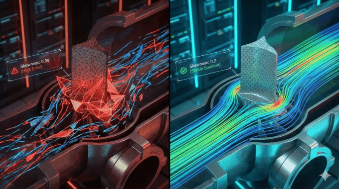
Why Metis? In a complex automotive geometry, a simple coordinate cut (cutting the car in half down the X-axis) often results in some cores having very easy work (open air) while others get bogged down with complex boundary layer cells. This creates a load balancing optimization failure—fast cores sit idle waiting for slow cores to finish.

Metis uses a graph-based algorithm to partition the mesh such that:

1. Every core gets an equal computational load (cell count is balanced).
2. The “interface” area between partitions is minimized.

Minimizing the interface is crucial because it reduces the amount of data that needs to be sent over the network (MPI communication). For this 120M cell case, switching to Metis improved the speed per iteration by an additional 12% compared to standard partitioning.

---

What Were the Speed-Up Results vs. a Standard Workstation? [The Benchmark]

The results of the migration to ansys hpc were transformative. We tracked the wall-clock time per time-step after the flow had stabilized to ensure fair benchmarking methodology.

Comparative Benchmark Results:

Metric	Local Workstation (32 Cores)	MR CFD HPC Service (512 Cores)	Speed-Up Factor
Memory Status	Swapping (Paging) to Disk	100% In-RAM	N/A
Time Per Iteration	~2,700 seconds (45 min)	6.5 seconds	415x
Time Per Time-Step	~4.5 hours	39 seconds	415x
Est. Total Project Time	~10.2 Years (Impossible)	~9 Days	Business Critical

Note: The speed-up here is higher than linear scaling because we eliminated the memory swapping bottleneck. Once the swapping stopped, the pure compute speed-up from core scaling kicked in.

You can access similar power through our ansys hpc services.

---

Did the Simulation Achieve Linear Scalability Across 512 Cores?

A critical part of our linear scalability validation was checking if we were getting good value for the core count. If you double the cores, you ideally want double the speed.

We performed a scaling study from 64 cores up to 512 cores on the cluster.

• Ideal Scaling: 100% efficiency.
• Actual Efficiency at 512 Cores: 88%.

An 88% MPI parallel efficiency at this scale is excellent. It demonstrates that the interconnect latency analysis held up—the InfiniBand network was fast enough to handle the communication chatter between 512 independent processes without becoming a bottleneck. This proves that Ansys Fluent scales remarkably well for large unstructured meshes when supported by enterprise-grade infrastructure.

---

What Is the Business ROI of Switching to On-Demand HPC?

For our client, the ROI wasn’t just about saving time; it was about saving the project.

1. Reduce Simulation Turnaround Time: They moved from a timeline of “impossible” to “under two weeks.” This allowed them to meet their certification deadline.
2. Zero CapEx: Building a 512-core cluster with InfiniBand would have cost them upwards of $150,000, plus months of procurement and setup. Using MR CFD’s cloud supercomputing for engineering, they paid a fraction of that cost as an operational expense (OpEx).
3. Higher Fidelity: Knowing they have this compute power on tap, the client has permanently upgraded their standard mesh settings. They no longer compromise on physics to fit a workstation.

---

How Can You Access MR CFD’s Managed HPC Services Today?

You do not need to be a Linux expert or a cluster administrator to get these results. We have designed our service to be as seamless as possible.

1. Book a Consultation: We review your .cas file and recommend the optimal core count.
2. Upload & Launch: You upload your files to our secure, encrypted portal.
3. Monitor & Scale: We handle the scaling Ansys Fluent on cloud infrastructure. You simply watch the residuals converge.

Don’t let hardware limitations dictate the quality of your engineering. Experience the power of ansys hpc and request your trial today.

---

Frequently Asked Questions

How does Ansys HPC licensing work on your cloud service?

We offer flexible options. If you already own Ansys HPC Pack licensing, you can “Bring Your Own License” (BYOL) by connecting our cluster to your license server via a secure VPN. Alternatively, for clients without sufficient licenses, we can provide on-demand licensing for the duration of your project, ensuring you are legally compliant without purchasing permanent assets.

Is my data secure when uploading proprietary designs to MR CFD?

Security is paramount. We utilize industry-standard AES-256 encryption for all data transfers. Your simulations run in isolated containers or Virtual Private Clouds (VPCs), meaning no other user can access your compute nodes. Furthermore, we are happy to sign NDAs (Non-Disclosure Agreements) to guarantee the confidentiality of your intellectual property.

What is the minimum mesh size required to see benefits from HPC?

While Ansys HPC is powerful, it has a “start-up cost” due to network communication. Generally, we recommend roughly 50,000 to 100,000 cells per core for maximum efficiency. Therefore, a model under 2 million cells may not see significant speed-up beyond 32 or 64 cores. The massive scaling benefits (100+ cores) are best realized on meshes larger than 10 million cells.

Can I monitor the Ansys Fluent residuals in real-time?

Yes. You do not have to wait for the job to finish to know if it’s working. Our MR CFD managed HPC services include remote visualization capabilities. You can log in to a virtual desktop, open the Fluent GUI while the solver is running, and check residuals, monitor points, and even visualize flow field contours in real-time.

How do you handle large file transfers for results?

For a 120M cell case, the result files can be gigabytes in size. Instead of downloading everything, we recommend performing post-processing (rendering videos, contours, and streamlines) directly on the cloud using our remote desktop nodes. You then only download the lightweight images, videos, or CSV data, which saves hours of transfer time. If you must download the full data, we use advanced compression to minimize the file size.