Discrete Phase model (DPM): Particle Motion & Life Cycle
Introduction
In this article, we investigate the motion of a particle from its injection to its final probable destination.
Particle Motion
In a separate article, the trajectory calculations were discussed briefly. The governing equation on the discrete phase in general form is shown below:
: Particle Motion &Amp; Life Cycle 1")
As the particles are injected, their velocity and location should be determined in every time step in order to track them. There are two governing equations in particle transfer from current to next point:
: Particle Motion &Amp; Life Cycle 2")
After integration over time from the second equation, velocity and location of particle could be caught in the next step:
: Particle Motion &Amp; Life Cycle 3")
It must be noted that the amount of ![]() is the critical factor in the accuracy and speed of the simulation.
is the critical factor in the accuracy and speed of the simulation.
Particle Life Cycle
A particle’s life cycle starts the moment the injection occurs, then passes through the elements and finally reaches a boundary, or its fate somehow finishes.
: Particle Motion &Amp; Life Cycle 5")
- The injection point is the initial point where the particle is injected into the domain. There are different injection methods available in Ansys Fluent software.
: Particle Motion &Amp; Life Cycle 6")
- After passing through a cell(previous cell), the particle gets to the boundary between the previous and current cell while its properties update.
- The particle is at the previous cell’s exit surface and entry of the current cell.
- While tracking through the current cell, all defined properties of the particle will update every time step.
In detail, the definition of the time step in the Discrete Phase Model and all the possible methods to define / for the continuous and discrete phase are described in ‘Particle Tracking Option.
- At this point, the particle passes through the exit surface of the current cell and enters the next one while its position and properties are updated based on the defined time step.
- In the end, the trajectory of the discrete phase will finish in different probabilities:
- Outlet: ‘Escape’ type boundary condition
- Wall: ‘trapped & reflect’ type boundary condition
- Incomplete
: Particle Motion &Amp; Life Cycle 6")
Discrete Phase Particle’s fate
- Reflect
After the collision with the wall, the particle will rebound off, while there will be changes in the particle’s momentum.
- Trap
This boundary condition is for walls too. The particle trajectory will be terminated after the particle hits the wall. If the discrete phase is ‘evaporating droplets,’ its mass will enter the adjacent cell of the boundary as a vapor. Finally, if the discrete phase is ‘combusting particles,’ the remaining volatile mass will change to vapor.
- Escape
The inlet and outlet boundary conditions could be ‘escape.’ After reaching the escape boundary, the particle will pass it, and in other views, the trajectory calculation for that particle will be terminated.
- Wall-jet
This boundary condition is used for the walls with a high temperature so that liquid wall film cannot form there.
- Wall-film
To define walls in which the model of the liquid film is significant.
- Incomplete
Although this item is not a boundary condition, it could be the fate of the particles if they reach the maximum number of allowed time steps defined in Max. Number of Steps as shown below:
: Particle Motion &Amp; Life Cycle 7")
*The trajectory calculations of the particle will be terminated in this state.
Related Posts
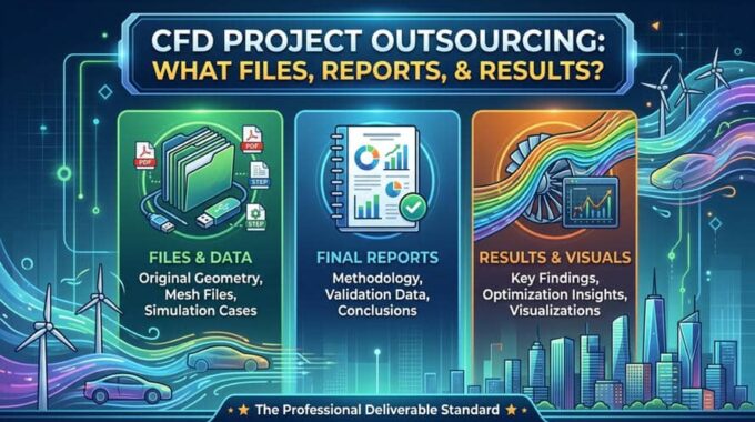
CFD Project Outsourcing: What Files, Reports, and Results Should You Expect?
When engineering teams decide to outsource CFD simulation, the conversation almost always starts with capability and…
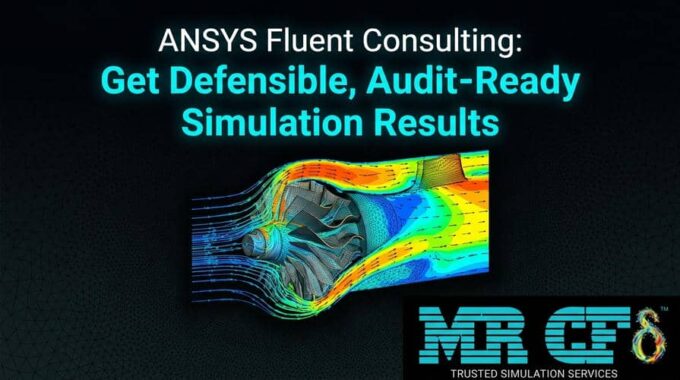
ANSYS Fluent Consulting: Get Defensible, Audit-Ready Simulation Results
You need ANSYS Fluent results that can survive scrutiny — a design review, a client…
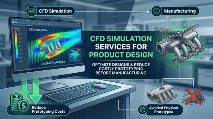
CFD Simulation Services for Product Design: Reduce Prototyping Cost Before Manufacturing
In modern product development, the most expensive mistakes are often discovered after money has already…
Comments (0)