Species Transport

What is Species Transport?

Convection, diffusion, and chemical reactions all contribute to the movement of different chemical species in a fluid flow, and these processes can be modeled and numerically simulated using computational fluid dynamics (CFD). Predicting the distribution of chemical species in a fluid flow can be done with the species transport equation, which is a convection-diffusion equation. In doing so, it considers

The transmission of chemical species as a result of the bulk motion of the fluid is called convection. Diffusion is the process by which a chemical species moves from a high-concentration to a low-concentration area. A reaction is a process by which new chemical species are formed or old ones are broken down.

Common forms of the species transport equation include:

∂(ρYi)/∂t + ∇•(ρYiU) = ∇•(ρDi∇Yi) + Ri

Where:

– ρ is the fluid density

– Yi is the mass fraction of the i-th species

– U is the fluid velocity vector

– Di is the diffusion coefficient of the i-th species

– Ri is the net rate of production of the i-th species due to chemical reaction

Many important engineering applications, including combustion, pollutant dispersion, and chemical reactor design, rely on solutions to this equation to forecast the distribution of chemical species in a fluid flow.

How can Species Transport CFD simulation be applied in Engineering and Industries?

The Movement of Species Many engineering and manufacturing areas rely heavily on CFD simulations. Some prominent uses include:

Combustion Science & Technology

Combustion engineers employ species transport simulations to foretell how fuel, oxidizer, and byproducts of combustion will be distributed inside a reactor. This is fundamental for developing clean and efficient combustion systems like automobile engines and power plant turbines.

Engineering for the Environment

Predicting how contaminants will move through the air or water is a common task in environmental engineering, and this is where species transport simulations come in. This aids in quantifying the environmental effects of manufacturing processes and developing pollution prevention strategies.

Chemical Engineers

Chemical reactors are designed and optimized with the help of species transport simulations in chemical engineering. The reaction’s rate and yield are affected by how the reactants and products are distributed within a reactor.

Engineering for the Medical Field

Species transport models are used in biomedical engineering to model the distribution of medications and other compounds within the body. This is significant for the development of drug delivery systems and the analysis of disease development.

The Food Industry

Species transport simulations are used to model the transfer of heat and moisture during cooking and drying processes in the food processing sector. As a result, food quality and safety can be improved.

The Oil and Gas Sector

The movement of oil, gas, and water through reservoirs and pipelines is modeled using species transport simulations in the oil and gas sector. This aids in maximizing oil and gas production and distribution.

Just a fraction of the various engineering and industrial uses for species transport CFD simulations include the ones listed above. Many industrial operations and environmental phenomena rely on our capacity to forecast the distribution of chemical species in a fluid flow.

MR CFD services in the Species Transport Simulation for Engineering and Industries

With several years of experience simulating various problems in various CFD fields using ANSYS Fluent software, the MR CFD team is ready to offer extensive modeling, meshing, and simulation services. Simulation Services for Species Transport CFD simulations are categorized as follows:

• Simulation and analysis of Virus Spread due to different phenomena and places.
• HVAC CFD Simulation in the operating room, smoking room, etc.
• Modeling of Combustion inside Storage Tank, Combustion Chamber, boiler, etc.
• Simulation of Providing Indoor and Outdoor Locations Thermal Comfort.
• Analysis of different Species applications in a fluidized bed, packed bed, etc.
• CFD Simulation of material decomposition.
• Analysis of Food Processing in case of drying, Refrigeration, etc.
• …

MR CFD is a leading provider of Computational Fluid Dynamics (CFD) simulation services for various engineering applications and industries, including species transport simulations. Here’s how MR CFD can assist:

Customized CFD Simulations

MR CFD offers customized CFD simulations based on the specific requirements of your project. This includes modeling complex geometries, multiphase flows, chemical reactions, and species transport.

Expert Consultation

MR CFD provides expert consultation to help you understand the CFD simulations’ results and guide you in making informed design decisions.

Training and Support

MR CFD offers training and support in using CFD software and interpreting simulation results. This can help you build in-house capabilities for CFD simulation.

Optimization Services

MR CFD provides optimization services to help you improve the performance and efficiency of your designs. This includes optimizing flow patterns, heat transfer, and species distribution.

Wide Range of Applications

MR CFD has experience in various applications, including combustion engineering, environmental engineering, chemical engineering, biomedical engineering, food processing, and the oil and gas industry.

In summary, MR CFD can provide comprehensive services in species transport simulation, from initial setup and simulation to result interpretation and Optimization, for a wide range of engineering applications and industries.

Humidification Dehumidification (HDH)

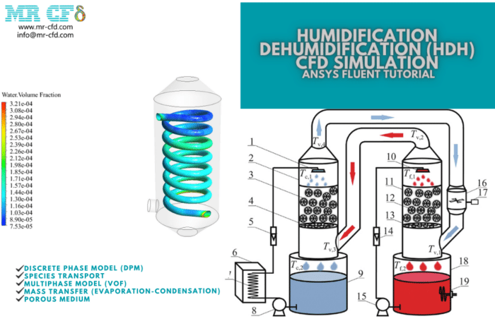
This CFD project uses the ANSYS Fluent software to discuss the humidification dehumidification (HDH) system. A good example of a water desalination system is the HDH system. The humidification and dehumidification processes form the basis of this method’s mechanism. The evaporator, or humidifier, is on one side of the system, while the condenser, or dehumidifier, is on the other.

The dehumidifier’s (condenser) spiral tubes are where the cold water enters. The steam inside the shell is then used to heat the water. The water inside the tube continues to receive heat until the steam condenses, at which point it is heated. This heated water enters the humidifier (the evaporator) and is sprayed onto the evaporator’s filter plates.

Wet steam or humidified air is created when these droplets are combined with the dry air that exits the condenser. Pure steam is produced, and any impurities settle to the bottom of the evaporator. A heater reheats this pure steam before it enters the condenser.

As previously indicated, the condenser shell’s interior is now in touch with the cold feed water pipes. The steam is humidified, or purified water is distilled from it. The two steps of the system’s process are humidification and dehumidification. For this issue, two simulations have been run. In the first simulation, humidification was studied. Dry air rises from the chamber’s bottom to its top. Hot salt water is sprayed via several pores inside the chamber simultaneously. After evaporating, the droplets in the membrane portion of the chamber clash with the airflow to create humid air.

This steam is salt-free and unadulterated. Dehumidification was the subject of the second simulation. The chamber is filled with the flow of moist air produced in the previous phase. Spiral tubes are thought to transport the cooling water flow inside the chamber. Freshwater is produced when hot steam touches the spiral tube’s cold surface and condenses.

The contours relating to the mass fraction of air and water vapor and the concentration of discrete particles have been acquired following the conclusion of the first simulation. The results only apply to the final second of the simulation because it is unstable.

Two animations have also been created to better comprehend the solutions to this challenge. On a two-dimensional plane, one looks at the contour of changes in the mass fraction of produced water. The compartment is being traversed by the plane. The other uses particle tracking to examine how water droplets spread over time.

The findings demonstrate that droplets are routinely shot downward from the chamber’s higher apertures in preparation for meeting dry air. The outcomes additionally demonstrate that water is gradually created over time and travels toward the upper exit of the chamber. Given that the purpose of the simulation was to produce humid air, this demonstrates that it was done correctly. Additionally, the mass fraction of produced water over time has been plotted. This plot demonstrates how steam builds up over time.

After the second simulation, it was possible to generate two-dimensional contours for the following variables: velocity, Temperature, mass transfer rate (from steam to water), and volume proportion of water and steam. This simulation has been running continuously and without regard to time.

The findings demonstrate the phase transition in the areas surrounding the cold spiral tube. The temperature contour reveals that the vapor temperature has dropped and fallen below the saturation point near the cold pipe. Condensation, or the conversion of vapor to water, must therefore occur.

The mass transfer rate’s contour also effectively demonstrates that the phase transition occurs in areas where the temperature is lower than the saturation temperature. When a phase transition from liquid to vapor occurs, the sign changes from negative to positive (indicating the phase transition from liquid to vapor). The contour of water and vapor volume fraction changes also confirm condensation. The results show that the areas closest to cold pipes are where the most produced water is found.

Population Balance Model for Nucleation (PBM)

The current issue uses the ANSYS Fluent program to simulate Calcium-Oxalate generation utilizing a Population Balance Model (PBM). We carry out this CFD project and do a CFD analysis to look at it. Following the simulation, two-dimensional findings about the mass fraction of the current chemical species at various times and for various bin numbers are obtained.

For instance, a two-dimensional contour is formed about the volume fraction of the primary phase, which includes water, calcium, and oxalate, and the second phase (calcium-oxalate). These contours demonstrate that a chemical reaction and mass transfer from the primary to the secondary phase are responsible for the formation of calcium oxalate. The initial chamber region, the intersection of two intake pipes, is where the desired material is formed.

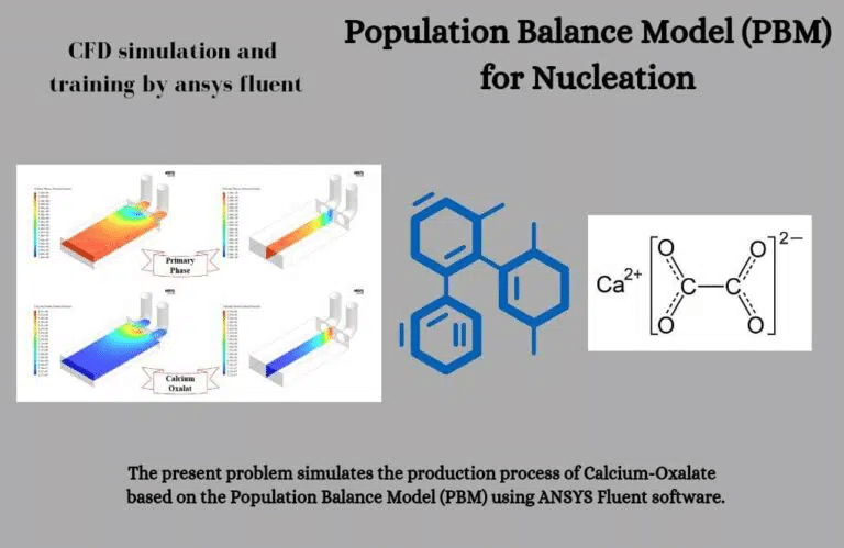
The table listing the dimensions of each definition category (bin) is then displayed. There are 48 categories for particle size classification, with bin-47 having a minimum size of 5e-7m and bin-0 having the largest size. Additionally, we use the bin number to show the number density bar graph.

The number density shows how many particles there are per unit volume or how many particles fit into the appropriate area, given the size of each bin. A two-dimensional contour of the volume fraction of calcium-oxalate produced in various bins is what we finally get. The findings indicate that the amount of material produced increases starting about bin-30.

This indicates that the amount of particles created in the bin-0 to bin-30 categories is negligible. The generated particles are formed and grow in smaller volumetric sizes (between bin-47 and bin-30) and are therefore undetectable in larger volumetric sizes, we can infer.

SOFC (Solid Oxide Fuel Cell) 

This project uses the ANSYS Fluent software to numerically simulate a solid oxide fuel cell (SOFC). An apparatus that transforms fuel energy into electrical energy is a fuel cell. The industry uses various fuel cell types, including SOFC, PEMFC, etc. In this project, a solid oxide fuel cell is modeled. This fuel cell can function in extremely hot conditions.

The cathode and anode are the two components that make up a solid oxide fuel cell. The electrolyte layer in the center of the fuel cell connects these portions. Each cathode and anode segment contains two layers of electrode and collector. The collectors function to conduct electric current and are built of solid material. These current collectors have a gas tube inside of them. The fuel cell is filled with hydrogen (or fuel) from the gas channel of the anode collector and oxygen (or air) from the gas channel of the cathode collector.

Ion conductive and porous electrode layers. In the cathode electrode, the oxygen reacts with free electrons to form positive ions. On the other side, hydrogen reacts with oxygen ions and free electrons in the anode electrode and forms water. Ceramic makes up the middle electrolytic layer, which conducts oxygen ions. These liberated electrons produce an electric current through the collectors and the circuit attached to the cell.

Following the computations, we are left with two-dimensional outlines representing the mass fraction, concentration, and combination of oxygen, hydrogen, and water. These contours accurately demonstrate how the fuel cell’s electrochemical reactions take place.

According to the findings, hydrogen and oxygen enter from the anode and cathode, respectively. Although there wasn’t any water within the fuel cell at first, the results indicate that it has formed on the anode side. This indicates that the fuel cell’s electrochemical process involving oxygen, hydrogen, and electrons has occurred.

We also measure the inside of the fuel cell’s electric potential and current contours. These lines accurately depict how electric current is produced. A current of electricity is produced inside the fuel cell due to the potential difference between the cathode and anode sides. Therefore, we can conclude that the solid oxide fuel cell system is functional.

Combustion in the Presence of EHD

Utilizing ANSYS Fluent, the current simulation deals with combustion in the presence of EHD. This assignment involves designing a straightforward combustion chamber. Air and fuel enter the combustion chamber’s cylindrical shape axially. So that air flows around C10H22 and enters the chamber from the center. Two stages were taken to complete this project. The investigation begins with a simple combustion between air and fuel. The same combustion is then carried out with an electrohydrodynamic (EHD) present.

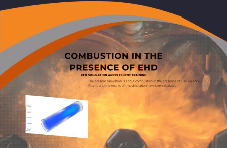
Fluids become charged when EHD is applied to them. How ionized particles or molecules move and engage with the electric field and surrounding fluid is investigated. The Species Transport model must be applied to define the combustion reaction. Calculations are performed to produce 2D and 3D contours of the species’ Temperature, velocity, pressure, and mass fraction (CO2, C10H22, O2, N2, and H2O). These results are shown in two different modes—without EHD and with EHD—so that the impact of the electric field can be investigated by contrasting the outcomes.

According to the contours, more heat is applied to the species in the combustion chamber when EHD is used, which raises the Temperature of the finished product. The combustion process happens more quickly as the Temperature of the reactive species rises. Additionally, by observing the behavior of reaction byproducts, it may be possible to determine that the combustion reaction will be of greater quality when EHD is present.

Proton Exchange Membrane Fuel Cell (PEMFC)

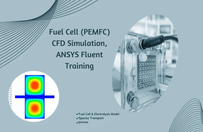
This research simulates a proton exchange membrane fuel cell using the CFD numerical simulation method and the ANSYS Fluent software. Fuel cells are less polluting than other forms of power generation since they produce energy through a chemical reaction. This project simulates a fuel cell using the PEMFC model.

The current study examines how a polymer fuel cell’s fluid behavior and thermal conductivity affect the mass fraction of gaseous species and the quantity of electricity generated in the cell. Results from the simulation are displayed as outlines when it has finished. The reaction between hydrogen and oxygen results in the creation of an electric current. Between the cathode and the anode, the electrolyte membrane serves as a bridge, while the catalytic layer increases transmission.

Combustion Chamber Performance Optimization, DOE

Design of Experiments (DOE), also known as Designed Experiments or Experimental Design, is the methodical process used in controlled settings to identify an unidentified effect, validate a hypothesis, or demonstrate a previously seen effect. It entails establishing the connection between the input variables influencing a process and its outcome. To maximize the result, process inputs should be managed.

The technique was first presented in the 1920s and 1930s by Sir Ronald A. Fisher. A robust technique for data collecting and analysis, experiments are designed in various experimental settings. It enables the manipulation of numerous input variables and the evaluation of their impact on the desired output (response). DOE enables discovery of significant interactions that could go undetected when exploring a single factor. The entire set of potential combinations, or just a portion, can be studied (full factorial).

A well-designed experiment may reveal a large quantity of information regarding the impact of one or more factors on a response variable. In many experiments, some variables are kept constant while the amounts of other variables are changed. However, this “one factor at a time” (OFAT) knowledge processing method is ineffective compared to simultaneously altering several factor levels.

Numerous methods can be used to implement DOE, as was previously discussed. Taguchi, Response Surface Methodology (RSM), Full and Fractional Factorial, and OFAT. However, among the currently used techniques for DOE, the RSM emerges as the most effective strategy.

A set of mathematical techniques known as the Response Surface Methodology, or RSM for short, is used to ascertain the link between one or more response variables and numerous independent (studied) variables. As a tool for experimental design, this approach was first presented by Box and Wilson in 1951. To create experimental models, RSM is a collection of statistical and applied mathematical methods. RSM aims to maximize the response, an output variable influenced by several independent variables. A set of tests known as executions make up an experiment. The input variables are altered in each experiment to identify the factors that led to changes in the response variable. Building response procedure models is an iterative process in response-level designs.

Once a rough model has been created, it is tested using the good-fit approach to determine whether the result is satisfactory. More experiments are run, and the estimating process is repeated if the solution is not verified. Experiment design aims to determine and examine the variables influencing the outcomes using the fewest possible experiments. This strategy produces the best response surface by identifying the ideal reaction level for each design variable. Experiment design aims to determine and examine the variables influencing the outcomes using the fewest possible experiments.

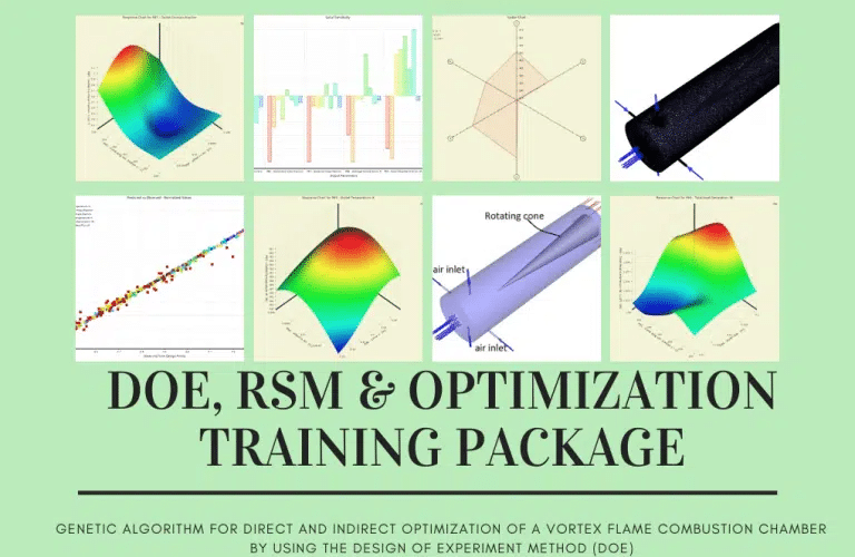
Optimization aims to find the optimal solution for a given parameter. One can carry out two different types of Optimization using ANSYS. Two types of Optimization exist: direct and indirect. The same solution will be obtained using either of these procedures but in a different order. Direct Optimization predicts how a system will behave without using any intermediate steps. Indirect Optimization, on the other hand, requires the information gathered by the RSM to give the user the right mathematical function for projecting system behavior.

The first section of this course, which seasoned engineers at MR-CFD wrote, will introduce you to various DOE approaches, including RSM and its background. The benefits or drawbacks of each method relative to the others will then be discussed, along with any theoretical underpinnings. Therefore, even if you have no prior knowledge of DOE or Optimization, you may be confident that you will learn the theoretical foundations you require in the introductory section.

The second section uses ANSYS software to carry out the RSM optimization procedure. This project will walk you through using this approach to tune various combustion chamber characteristics. For example, we will construct the shape of the combustion chamber from scratch and demonstrate how you may parametrize your design. In the following phase, you will observe how the meshing is carried out over the created geometry. We will then review how to install the Fluent program and establish additional necessary parameters. After that, we’ll demonstrate how to use a parameter correlation method to determine which input parameters significantly affect our output parameters. By removing the less-important input parameters, we may lower the number of input parameters and, consequently, our computation time.

Finally, by specifying the investigation span for each parameter, we build the design point chart using the Central Composite Method (CCD), a subset of RSM. This design point chart contains all the trials required for Optimization. Indirect Optimization in ANSYS, to put it simply, leverages the data produced by RSM to extract a mathematical function that can forecast the system’s behavior.

The direct optimization procedure is thoroughly detailed in the next section. As opposed to the previous method (RSM), this type of Optimization creates design points depending on the requirements of the software and a specified algorithm. The software can decide to forecast the mathematical function of the system effectively. It needs additional sampling points as the optimization process moves forward. To put it another way, in contrast to Optimization using RSM, the entire Optimization is carried out without the need for any intermediary steps. Finally, once the procedure is complete, ANSYS will give you three candidate points that, given the user-defined objective(s) (i.e., the conditions you want your model to satisfy), are the optimum solutions for your system.

This project simulates the combustion process inside a combustion chamber while monitoring variables like the rate of heat creation, pollution production, etc. (The following table displays the input and output parameters list.) The goal of this project, as described in the preceding paragraphs, is to optimize the geometrical characteristics of the combustion chamber to achieve objectives like optimizing the heat generation rate while limiting the amount of generated pollution. Indirect Optimization utilizing the RSM approach and direct Optimization are also addressed in this project. In the indirect optimization step, we use the CCD approach to create the design points required for the RSM analysis. The best input parameters for our model will then be determined through a parameter correlation procedure.

The input settings for the combustion chamber will then be optimized based on the data produced for the RSM analysis. The steps for performing direct Optimization are demonstrated in the second section. First, we will generate the design points required for the optimization process. Then, by specifying the desired target(s) (for example, maximizing the value of the heat generation rate while minimizing the amount of formed pollution), the software will begin the optimization process and give you the top three candidate points.

Equations relating to turbulent fluids are solved by using the RNG k-epsilon model. The temperature change can be calculated, and the heat transfer can be modeled using the energy equation. The species transport model and the volumetric response option have both been activated to mimic the combustion process inside the cylindrical combustion chamber.

The goodness of fit graph shows a good agreement between the projected values (predicted function) and the simulated points. As a result, you can rely on the collected data to provide you with the input-based ideal values for each outlet parameter. To visualize the results more clearly and comprehend the interactions between each input parameter and the output, you can extract a variety of 3D surfaces.

It is possible to determine which input parameter significantly impacts outputs by looking at the local sensitivity chart. For instance, it is clear from this study that the outer diameter and cone angular velocity of the combustion chamber influences practically all of the output characteristics.

Finally, you can see the replies for each parameter in the spider chart. (i.e., when the values of parameters 1, 2, 4,5, and 6 are at their highest, the value of parameter three will be at its lowest.) This is rational because, in a fully stoichiometric process, the mass fraction of CO will be zero while the generated heat will reach its highest value.

Polymer Electrolyte Membrane Fuel Cell (PEMFC)

The current issue uses the PEMFC (polymer electrolyte membrane fuel cell) model to mimic a fuel cell in a porous media. There are two primary cathode and anode segments in the model. Each consists of four layers: a flow collector, a flow channel, a gas distribution region, and a catalytic section. The polymer membrane fills the space between the anode and cathode layers.

This study looks into a polymer fuel cell’s fluid behavior and thermal conductivity, how they affect the mass fraction of gaseous species, and the quantity of electricity generated in the cell. Results from the simulation are displayed as outlines when it has finished. The electrolyte membrane allows the transfer of hydrogen and oxygen ions as expected. The catalyst might also speed up the process, causing the reactions to happen more quickly and producing an electric current.

Circulating Fluidized Bed (CFB) Gasifier

The Circulating Fluidized Bed gasifier is popular in commercial applications and academic investigations because of its inherent benefits in high circulating rate, low operating temperature, wide fuel flexibility, and negligible pollutant emissions. This simulation involved simulating a straightforward CFB cycle and obtaining results.

The system has two inlets: a vertical inlet for the oxidizer and a horizontal inlet for the fuel. After the air and fuel are mixed, flameless combustion begins in a vertical section; after entering the cyclone to separate unburned ashes from polluted air, the unburned fuel circulates to the bottom of the downstream section and enters the process again. Heavy sands and ashes exit from the bottom outlet. This simulation of solid dynamics uses the particle density function (PDF).

As a result of the fuel-air mixture igniting in the vertical chamber, hot gases from the ignition were cooled in the cyclone and the second chamber and the maximum face’s polluting gases were also investigated, according to the simulation results. The cyclone separates unburned components, which are added to the combustion process.

Population Balanced Model Crystallization

A fundamental phenomenon is the crystallization process, in which solute particles combine to form a solid crystal structure. A population balance model (PBM) can be used to model the crystallization process and provide a thorough understanding of crystal development, nucleation, and size distribution. It takes into account temperature, contaminants, supersaturation, and mixing circumstances. Researchers can simulate and forecast the behavior of crystals during the crystallization process by resolving the population balance equation.

Population balance modeling of the crystallization process offers important insights into crystal development, nucleation, and size distribution. This strategy has applications in the chemical, culinary, materials science, pharmaceutical, and energy storage industries. By comprehending and managing the crystallization process, researchers can improve product quality, increase process effectiveness, and contribute to improvements in various industrial industries.

As seen, many contours are displayed, including the distribution of various classes of bins, changes in the fraction of each bin, and the velocity of the phases inside the domain. The interaction between the Ca and Carbonate ions occurs precisely over the line where the two ions are combined, according to the heterogeneous reaction contour. Additionally, consider viewing the outlines of various bin classes. The volume fraction of each bin has increased in the domain in that scenario, showing the formation of the solid phase of calcium carbonate, making it simple to comprehend how the nucleation and growth phenomena have operated. Consider, too, that the number density histogram plot is shown. In that instance, it is clear that more bins may be used and that smaller bin sizes may be considered because the number density is almost zero.

In comparison, the smallest bin has a very high number density. This can be taken to mean that not all tiny bins and particles are taken into account. As a result, this issue can be resolved by using smaller values for the minimum diameter in the PBM settings.

Revolving Rice Dryer Using DPM

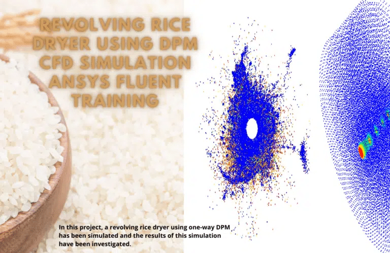
In this research, a rotating rice drier device was simulated using the Ansys Fluent software’s Evaporating droplets with a one-way DPM model, and the results were then examined. The large chamber’s center has a porous tube with holes via which hot air enters the rice dryer. In a chamber rotating at 100 rpm, three million rice grains are injected with 15% moisture droplets.

They assemble around the porous tube in the chamber’s center after being injected with around three million rice particles through the entrance. As seen in Figure 1, the H2O mass fraction initially gathered around the tube, but over time, due to the hot air being released from the tube holes into the chamber, the evaporating process started and caused the H2O to disperse; this may reduce the moisture of the rice particles, which was 15% initially, and as a result, the diameter decrease that is shown in figure 2. Additionally, the chamber’s rotational speed quickens the flow of heated air.

How to Model Species Transport inside ANSYS Fluent

Modeling species transport in ANSYS Fluent involves several steps. Here is a step-by-step guide:

Step 1: Create the Geometry and Mesh

First, you need to create the geometry of your system in CAD software and then import it into ANSYS Fluent. After importing, you need to create a computational mesh. The quality of the mesh can greatly affect the accuracy of your simulation.

Step 2: Define the Material Properties

Next, you need to define the material properties of the fluid, including its density, viscosity, and specific heat. If you are modeling multiple species, you need to define the properties of each species.

Step 3: Set Up the Species Transport Model

In the ‘Models’ menu, select the ‘Species’ model. Depending on your system, you can choose between different options, such as ‘mixture’ or ‘multicomponent.’ You must also specify the reactions, if any, and the reaction rate.

Step 4: Set Up the Boundary Conditions

In the ‘Boundary Conditions’ menu, you need to specify the conditions at the boundaries of your system. This includes the inlet conditions (such as the flow rate and the species concentrations) and the outlet conditions.

Step 5: Initialize the Solution

In the ‘Solution Initialization’ menu, you must provide initial guesses for the flow field and the species concentrations. You can usually start with a uniform flow field and uniform concentrations.

Step 6: Run the Simulation

Finally, you can run the simulation. During the simulation, ANSYS Fluent will solve the species transport and fluid flow equations to predict the species distribution in your system.

Step 7: Analyze the Results

After the simulation, you can analyze the results using the post-processing tools in ANSYS Fluent. This includes the visualization of the species distribution and the calculation of various quantities of interest. Remember, CFD simulations can be complex and require a good understanding of fluid dynamics and numerical methods. If you are new to ANSYS Fluent, consider getting training or consulting with an expert.

Ansys Fluent can simulate the mixing and transport of chemical species by resolving conservation equations defining the convection, diffusion, and reaction sources for each component species. It is possible to explain many simultaneous chemical reactions in the fluid phase (volumetric reactions), on wall or particle surfaces, or in the porous zone. This section describes the modeling capabilities for species transport, both with and without reactions.

Fluent can model species transport and reaction using several independent models.

• Species Transport and Finite-Rate Chemistry Approach
• Non-Premixed Combustion Approach
• Premixed Combustion Approach
• Partially Premixed Combustion Approach
• Composition PDF Transport Approach

Species Transport Approach

Convection, diffusion, and reaction sources conservation equations for many component species are solved using this method. Multiple chemical processes that occur in the bulk flow, at wall or particle surfaces, or in the porous zone can all be simultaneously specified by the user for modeling. Multicomponent transport inevitably introduces important physical effects, such as temperature gradients, enthalpy transmission, and diffusion. The reaction rate R_i may be specified as:

Finite-Rate model (Arrhenius kinetics)

General finite-rate chemistry directly determines reaction rates by ignoring the impact of turbulent fluctuations on kinetics rates.

Eddy-dissipation model

To avoid costly Arrhenius chemical kinetic calculations, reaction rates are believed to be controlled by turbulence while neglecting the impact of chemistry timeframes. The model is computationally cheap, but only one or two-step heat-release mechanisms should be utilized for realistic results. This strategy should only be applied when the chemistry timescales of interest are known to be quickly compared to the domain’s turbulence timescales.

Eddy-dissipation-concept model

Turbulent flames can incorporate complicated chemical kinetics while considering turbulence and kinetics timescales. It should be noted that detailed simulations of chemical kinetics might be computationally expensive. Diffusion- or kinetics-limited surface reactions are also possible; in the second case, surface coverage may also be important. In this situation, Fluent can monitor the molar concentrations of species that have adsorption to walls. Modeling of particle surface reactions is also possible.

Non-Premixed Combustion Approach

Instead of writing and solving transport equations for individual species, this method writes and solves them for mixed fractions. The resulting mixture fraction field is used to compute the species concentrations. The non-premixed combustion approach is predicated on the idea that you are simulating a diffuser or pulverized fuel flame, with all combustion systems having separate fuel and oxidizer inlets. The foundation of the non-premixed combustion model is that a fluid’s current thermochemical state can be connected to a conserved scalar variable.

Premixed Combustion Approach

Before ignition, fuel and oxidizer are molecularly combined in premixed combustion. A flame front spreading into the unburned reactants causes combustion to happen. A thin, spreading flame moves over the (potentially turbulent) boundary during premixed combustion. Non-premixed combustion is often a mixing issue in a contract. Tracking the turbulent flame speed as a function of the laminar flame speed and the turbulence at the interface is the main issue for premixed combustion.

Partially Premixed Combustion Approach

The Partially Premixed Combustion model is based on non-premixed and premixed combustion models. Systems that use partially premixed combustion produce flames with irregular fuel-oxidizer mixes with equivalence ratios. These flames include imperfectly premixed inlets, lean premixed combustors with diffusion pilot flames and cooling air jets, and premixed jets discharging into a still atmosphere.

Composition PDF Transport Approach

A probability density function (PDF) can be used by ANSYS Fluent software to explain finite-rate chemical kinetics in turbulent reacting flows. This method, for instance, can be used to model effects like flame extinction and ignition of species like NOx. Even though it requires complicated computation, this model has the advantage of sometimes accurately accounting for turbulent flow.

Combustion Training Course

You can identify as a Combustion CFD Simulation specialist after completing this Combustion Training Course. Fuel and oxygen undergo a high-temperature exothermic chemical reaction known as combustion, which typically results in gaseous byproducts like CO2 and water vapor. Typically, combustion is accompanied by flame—a combination of light, high Temperature, and tremendous energy release.

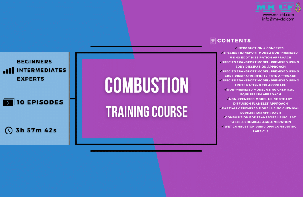
Since the first human discovered fire, combustion and fire have been the most important sources of energy he needs to survive, with modern uses in boilers, burners, furnaces, and other devices.

The quantity of fuel and oxidant needed in a boiler’s combustion chamber to produce a specific amount of energy required to run an electric plant is thus one of the fundamental features of combustion. In this regard, CFD is regarded as the most amazing instrument for forecasting and calculating the required amount of fuel and oxidant and forecasting the released energy.

An effective tool that can be useful is ANSYS Fluent. The software’s built models can foresee even the smallest changes in Temperature brought on by the combustion process and heat emission. As a result, CFD is regarded as a potent tool for modeling combustion and creating various and effective forms of combustion chambers. In this training course, you will learn how to configure the necessary settings for using the species transport model to model the combustion process in any domain.

Step-by-step instructions are provided on how to simulate the formation of pollution such as NOx, SOx, and soot in Fluent using a variety of simulation models and techniques, such as Finite rate (No TCI), Eddy dissipation, and Eddy dissipation/Finite rate. You will first learn the fundamentals of each model before learning strategies and pointers for carrying out precise and accurate combustion simulations. To ensure that the graduates can effectively use this program to produce high-fidelity combustion simulations after completing the training course, this course is delivered in a manner that is as practical as is practical.

Included in the combustion training course are:

• Introduction to combustion and an overview of available CFD simulation techniques and models in ANSYS Fluent.
• Non-premixed combustion modeling using the Eddy Dissipation
• Premixed combustion modeling using the Eddy Dissipation
• Pollution formation
• Premixed combustion modeling using the Finite rate/No TCI
• Non-premixed combustion with separate inlet boundaries for fuel and air by assuming Chemical Equilibrium among chemical reactants and products
• Non-premixed combustion inside a combustion chamber with separate inlet boundaries for fuel and air by assuming a steady diffusion flamelet
• partially-premixed combustion
• partial differential function (PDF) transport model combustion

Species Transport MR CFD Projects

MR CFD has a rich portfolio of projects related to species transport simulations. Here are a few examples:

Combustion Simulation in a Gas Turbine

In this project, MR CFD used ANSYS Fluent to simulate the combustion process in a gas turbine. The simulation included fuel and air species transport, chemical reactions, and heat transfer. The results helped to optimize the turbine design for better efficiency and lower emissions.

Air Quality Modeling in a City

MR CFD used CFD simulations to predict the dispersion of pollutants in a city. The simulation included the transport of multiple pollutant species, the wind flow, and the effect of buildings on the flow and dispersion. The results provided valuable information for urban planning and air quality management.

Air Pollution Ventilation Training Package

Five CFD tasks are included in this air pollution ventilation training package to explore smoke and automobile explosion pollutant ventilation employing jet fans in a tunnel, pollution ventilation in the subway, shuffle parking, and car park (stacker) ventilation.

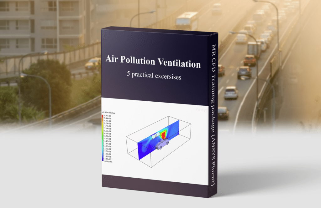
To assist you in comprehending the foundations of CFD and how to use it to solve air pollution ventilation problems, the program includes a thorough series of lessons and exercises. Additionally, a library of 3D models and meshes is provided to aid in creating your simulations. The program also has several tools to aid with data visualization and analysis of the simulation results.

Finally, the package includes several case studies clarifying how we apply CFD to address actual issues. Ventilation for air pollution Air flow in a specific environment can be simulated using the computer-aided engineering (CAE) technology known as CFD simulation. We use this simulation to examine how air pollution affects the ecosystem, including how pollutants spread, how wind affects air quality, and how well ventilation systems work.

The simulation can also improve the ventilation system design to reduce air pollution. Typically, we use computational fluid dynamics (CFD) software to run the simulation. Mathematical models are used in the simulation to mimic the airflow in a certain environment. The simulation’s findings can guide decisions on the layout and operation of ventilation systems and pinpoint potential air pollution sources.

Pollutant Dispersion into the Air, CFD Training Package

Six CFD tasks are included in this training package on pollutant dispersion into the air to explore the air pollution in street canyons and actual metropolitan areas, pollutant distribution from car exhaust in static and traffic (cars moving slowly) modes, and gas flares.

To assist you in understanding the foundations of CFD and air pollution modeling, the program offers a substantial collection of tutorials and tasks. The governing equations and boundary conditions applied in the simulations are also thoroughly explained. Additionally, the software offers a library of pre-built models and boundary conditions to facilitate speedy simulation setup and execution.

You can examine and display the outcomes of your simulations with a library of post-processing tools that is part of the Pollutant Dispersion into the Air CFD training package. To help you better understand the outcomes of your simulations, these tools also feature a variety of graphical and statistical analysis tools and a variety of visualization tools.

Finally, the program comes with a vast array of resources to assist you in comprehending the foundations of CFD and air pollution modeling. To assist you in comprehending the foundations of CFD and air pollution modeling, these resources contain a variety of books, articles, and videos.

CFD (Computational Fluid Dynamics) simulation can simulate how contaminants are distributed throughout the atmosphere. The simulation can also forecast the amount of contaminants in the air at various periods and locations. We utilize the simulation to assess the impact of several elements on the dispersion of contaminants, including wind speed, Temperature, and humidity. The simulation can pinpoint locations where pollutant concentrations are over permitted limits. Additionally, we use the simulation to locate the origins of the contaminants and create plans for lowering their output.

Reaction Engineering in a Chemical Reactor

In this project, MR CFD simulated the reactions and species transport in a chemical reactor. The simulation helped to optimize the reactor design and operation for better performance and higher yield.

Food Processing Simulation

MR CFD used CFD simulations to model the transport and reactions of different species during food processing. The simulation helped to improve the quality and safety of the food products.

Oil and Gas Applications

MR CFD has done several oil and gas-related projects, including simulating multiphase flows and species transport in pipelines, separators, and other equipment.

These projects demonstrate the wide range of applications of species transport simulations and the expertise of MR CFD in this field.

Species Transport Application in Industrial Companies

Species transport modeling plays a critical role in many industrial applications. Here are a few examples:

Petroleum Industry

In the petroleum industry, species transport modeling simulates the flow and mixing of different hydrocarbon species in pipelines, reservoirs, and processing equipment. This helps in optimizing the production and refining processes.

Chemical Industry

In the chemical industry, species transport modeling is used to design and optimize chemical reactors. It helps understand the reaction kinetics and predict the desired products’ yield.

Pharmaceutical Industry

In the pharmaceutical industry, species transport modeling is used to design and optimize drug delivery systems. It can help predict drug release and distribution in the human body.

Environmental Engineering

In environmental engineering, species transport modeling is used to predict the dispersion of pollutants in air and water. It helps assess the environmental impact of industrial activities and design pollution control systems.

Food Industry

Species transport modeling is used in the food industry to design and optimize food processing operations. It can help predict the changes in the composition and quality of food products during processing.

Semiconductor Industry

In the semiconductor industry, species transport modeling is used to design and optimize deposition and etching processes. It helps in controlling the composition and thickness of the thin films.

These are just a few examples. Species transport modeling is a powerful tool that can help industrial companies improve their processes, products, and environmental performance.

MR CFD Industrial Experience in the Species Transport Field

Some examples of Species Transport industrial projects recently simulated and analyzed by MR CFD in cooperation with related companies are as follows:

Ramjet Engine, Design and Combustion Optimization (SR-71 Blackbird)

Instead of using a rotary compressor, an air-breathing jet engine, a ramjet, compresses incoming air by propelling the engine forward. Ramjets cannot function at zero airspeeds. They cannot be used to propel an aircraft through all stages of flight. The aircraft needs extra propulsion to accelerate an aircraft with ramjets to a speed where the ramjets can deliver thrust.

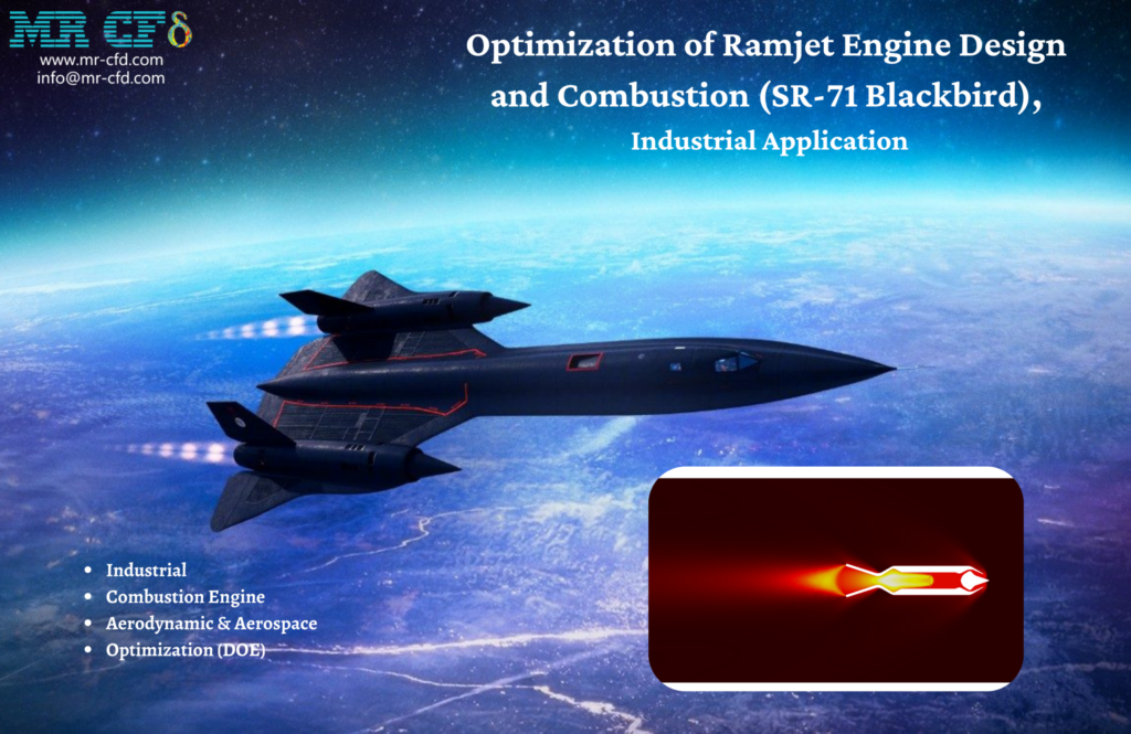
The combustion that produces thrust occurs at a subsonic speed in the ramjet’s combustor. A supersonic vehicle needs the aircraft inlet to slow the air entering the engine. Shock waves in the inlet cause performance losses in the propulsion system. Over Mach 5, ramjet propulsion is comparatively inefficient.

Fuel is essential in this scenario. Hydrogen is especially desirable because of its well-known, relatively short inflammatory delay when other positive aspects are taken into account, such as the fact that the air’s overall Temperature is high at high Mach numbers.

An SR-71 Black Bird traveling at a Mach number of 3.3 is considered in this simulation. The goal is to simulate the ramjet engine to understand what occurs there and explore the parameters. After three important parameters have been chosen, the solution is optimized in the following phase using the DOE approach in the ANSYS Workbench program.

The Design of the Experiment study is conducted on the solution to enhance device performance and obtain the highest possible fuel efficiency and, as a result, thrust number. Three parameters significantly impacting the outcomes are selected to study the consequences of their adjustments. These are the parameters:

1. Flow rate of fuel mass
2. Angle of injection
3. The separation between the engine inlet and the injection slot

The DOE model also provided the minimum and maximum values of the parameters, considering their interactions.

Improved greenhouse ventilation techniques

A greenhouse is a glass or plastic building that encloses a portion of a field from the outside environment. It offers cover and safeguards plants from extreme weather variations and obstructive elements like insects and animals, for instance, during excessively cold or hot seasons. Because of these constraints and amenities, constructing a greenhouse environment strives to offer delicate plants a secure and ideal atmosphere to grow gradually.

We looked into ventilation and design enhancement for greenhouses in this industrial project. The employer provided an inside greenhouse area plan. A reasonable temperature range, a high tolerable humidity level, and maximal ammonia reduction are crucial elements in this space’s ventilation.

This greenhouse’s basic layout includes two commercial fans. The MR-CFD simulation expert group did a numerical simulation in the first stage and evaluated the findings. The experts concluded that the current design is not by the three objective factors. Thus, fans alone cannot improve the greenhouse’s air quality.

The CFD team advised the client to mount a water-cooled air conditioner on the wall before the fans. Promising outcomes were reached in the simulation’s second step. Coolers have made a substantial contribution to improving air humidity and decreasing ammonia. The Temperature was still at the top limit; thus, this strategy proved ineffective.

This is because the cooling system, which is situated in the middle height of the room, cannot circulate the hot air, which builds up close to the greenhouse ceiling due to the buoyancy effect and stagnation. The simplest approach is to speed up the cooling system’s cold air, which is bad for greenhouse products. Therefore, the MR-CFD team advised the project’s client to relocate to where the water-cooled air conditioner will be installed. With this in mind, we began the simulation’s third step.

The third step’s outcomes were incredibly pleasant. By putting up the appropriate ideas, we could satisfy all three requirements. You might be curious about how the temperature range was constrained. Take note of the buoyancy effect and natural convection heat transfer. Warm air rises to the top of the atmosphere because it is lighter and less dense. As a result, hot air gathers close to the greenhouse’s roof.

It is now sufficient to mount the cooling system atop the inside of the greenhouse. The cooling airflow lowers the Temperature of the gathered air. Continuous air recirculation is produced because the air falls again as the temperature rises and the air becomes heavier.

Furnace

In this project, an industrial furnace was simulated, and ANSYS Fluent software was used to analyze the simulation findings. We carry out this CFD project and do a CFD analysis to look at it. The methane in the pipes is heated in the furnace that serves as the project’s model so that it can be moved more easily and with less effort.

The data demonstrate that methane pipes’ exit temperatures have risen relative to their entrance temperatures. Combustion starts when the fuel enters the furnace and mixes with the air. The furnace’s floor is covered with six burners. Methane, a liquid inside the pipe, is heated when the flame strikes the pipes in the radiant area of the furnace. Burnt gases from the combustion process are expelled from the chimney.

The oil, gas, and petrochemical industries use furnaces to supply heat for various activities that require temperatures above 400 C. It is frequently necessary to lower the viscosity of heavy mineral flood oil to facilitate this procedure by heating the oil in the furnace. To raise the Temperature of methane is the goal of this study.

In this study, an industrial furnace was numerically stimulated using ANSYS Fluent software. The methane in the pipes is heated in the furnace that serves as the project’s model so that it can be moved more easily and with less effort. The data demonstrate that methane pipes’ exit temperatures have risen relative to their entrance temperatures.

One of the priceless things that nature has bestowed on us is oil. It is impossible to overlook the influence of oil on humankind’s economic, political, and social domains. The development of the economy, creation of jobs, and peace have all benefited from oil as a necessary component.

The displacement of oil or its products in transmission lines, which are difficult to move in the pipeline due to their high viscosity, is thus one of the primary issues in the oil business. As a result, by heating the necessary fluid, the viscosity is reduced, improving the displacement in the tube.

Like other pieces of equipment, furnaces evolve with time, and as engineering knowledge has risen, so too have the efficiency and safety of new designs. When creating and designing various furnaces, engineers’ intellectual preoccupations include maximizing efficiency, enhancing safety, streamlining, providing direction, and enabling the use of various fuels in the furnaces.

Combustion starts when the fuel enters the furnace and mixes with the air. The furnace’s floor is covered with six burners. Methane, a liquid inside the pipe, is heated when the flame strikes the pipes in the radiant area of the furnace. Burnt gases from the combustion process are expelled from the chimney. The results show that an adequate flame has been created and that the Temperature of the pipes at the outflow has greatly increased compared to the intake.

---

You may find the Learning Products in the Species Transport CFD simulation category in the Training Shop. You can also benefit from the Species Transport Training Package, which is appropriate for Beginners (Part1 & Part2), Intermediate (Part1 & Part2), and Advanced users of ANSYS Fluent. Also, MR CFD is presenting the most comprehensive Species Transport Training Course for all ANSYS Fluent users from Beginner to Experts.

Our services are not limited to the mentioned subjects. The MR CFD is ready to undertake different and challenging projects in the Species Transport modeling field ordered by our customers. We even carry out CFD simulations for any abstract or concept Design you have to turn them into reality and even help you reach the best strategy for what you may have imagined. You can benefit from MR CFD expert Consultation for free and then Outsource your Industrial and Academic CFD project to be simulated and trained.

By outsourcing your Project to MR CFD as a CFD simulation consultant, you will not only receive the related Project’s resource files (Geometry, Mesh, Case, and Data, etc.), but you will also be provided with an extensive tutorial video demonstrating how you can create the geometry, mesh, and define the needed settings (preprocessing, processing, and postprocessing) in the ANSYS Fluent software. Additionally, post-technical support is available to clarify issues and ambiguities.