Errors Occurring in Simulations with ANSYS Fluent: A Technical Guide to Convergence & Stability

ANSYS Fluent simulates engineering problems based on the Finite Volume Method (FVM). Consequently, the errors generated by this software are inherently rooted in this numerical approach. While some errors may originate from the internal structure of the software or computational processing limitations, a significant portion of potential errors can be prevented before the solver is even run.

By addressing these issues early, engineers can not only achieve high-quality simulations and improved solution development but also significantly reduce computational costs. In this technical report which is continuously updated by the Mr CFD team, we investigate these errors thoroughly, sharing our experience to help you improve simulations and achieve accurate, converged results.

The 5 Main Categories of ANSYS Fluent Errors

To troubleshoot effectively, we must first categorize the errors generated by the software:

1. Convergence and Stability Errors (The most common and critical)
2. File and Import Errors
3. Initialization and Startup Errors
4. Solver and Batch Errors
5. Advanced Feature Errors

In the following sections, we will deep-dive into the first and most significant category: Convergence and Stability, providing valuable solutions for resolving these critical issues.

---

Deep Dive: Convergence and Stability Errors

Convergence failure is the most frequent hurdle in CFD. Divergence means the solver is unable to establish a balance among mass, momentum, and energy transport.

• Physical Perspective: The flow experiences sudden, extreme acceleration or produces unrealistic temperature/pressure values.
• Numerical Perspective: The discretization scheme fails to correctly represent gradients.

We have categorized the primary causes of these instabilities into five specific sub-groups:

1. Diverging Simulations (General)
2. Unphysical Results
3. Turbulent Viscosity Ratio Exceeded
4. Not a Number (NaN) and Infinity
5. AMG Solver Divergence

---

1. Diverging Simulations: Root Causes & Solutions

In a divergent simulation, residuals grow uncontrollably instead of decaying. This is rarely due to the algorithm itself, but rather inconsistencies in the physical model, grid quality, or numerical settings.

A. Poor-Quality Computational Mesh

The Cause:

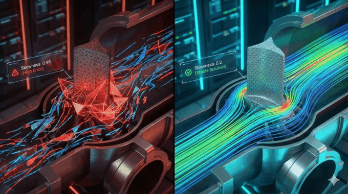
The quality of your mesh is the single biggest factor in simulation stability. Cells with very high Aspect Ratios or severe Skewness lead to numerical instability in diffusion and convection processes.

• Example: High skewness causes the surface normal vector to deviate from the true flux direction. This leads to incorrect calculations of diffusive gradients, resulting in non-physical oscillations.

The Solution:

Strictly evaluate mesh metrics during generation.

• Aspect Ratio: Ideal is < 100.
• Skewness: Ideal is < 0.5. Values up to 0.94 are generally acceptable for simple flows.

Critical Note on Flow Physics:

Acceptable ranges depend entirely on the flow regime.

• Laminar Flow: May converge with skewness > 0.95.
• High Turbulence: May fail even at skewness of 0.85.
• Multiphase: Requires the strictest standards.

Error Distribution:

It is not just about the maximum skewness, but the location.

• Clustered Bad Elements: If low-quality cells are grouped together, divergence is almost guaranteed.
• Distributed Bad Elements: If they are isolated, the numerical instability is often damped by surrounding good mesh.

B. Wrong Boundaries

The Cause:

Incorrect boundary definitions force the solver into a mathematical contradiction.

• Example 1 (Compressibility): Filling a tank with gas defined as “incompressible” without an outlet.
• Example 2 (MRF): In a centrifugal pump simulation, failing to define the interface between rotating and stationary regions causes fluid to be “trapped,” leading to immediate divergence.
• Example 3 (Ejectors): In supersonic ejectors, a high-pressure inlet drives suction at a low-pressure inlet. If initialized incorrectly, flow may exit the low-pressure inlet instead of entering.

The Solution:

• Ejector Tip: Initially treat the low-pressure inlet as a wall. Allow the supersonic shock to form at the high-pressure port, then switch the wall to a pressure inlet.
• Check Consistency: Ensure physics (compressible vs. incompressible) match the boundary types (pressure outlet vs. wall).

C. Aggressive Under-Relaxation Factors (URFs)

The Cause:

URFs control how much the variable changes from one iteration to the next. “Aggressive” (high) URFs in problems with strong non-linearities or shocks cause variables to overshoot the physical solution, leading to wild oscillations.

The Solution:

• Start with conservative (low) URFs.
• If initialization is poor, drastically reduce URFs for the first 50-100 iterations.
• Gradually increase them once the flow field stabilizes.

D. Large Time Step Size

The Cause:

In transient simulations, a time step that is too large violates the Courant-Friedrichs-Lewy (CFL) condition. The solver cannot capture the physical changes occurring within that time frame.

The Solution:

• Use Adaptive Time Stepping.
• Monitor the Courant Number. For complex unstable problems, keep the Courant number very small (< 1) initially, then ramp up as the flow develops.

---

2. Unphysical Results

Sometimes residuals converge, but the data is wrong (e.g., negative temperatures, Mach 50 velocity).

The Cause:

• Inconsistent Physics: Using a turbulence model inappropriate for the Reynolds number.
• Combustion Errors: In species transport, if reaction rates or energy release parameters are incorrect, temperatures can skyrocket, causing the simulation to stop.
• Reference Values: Incorrect Operating Pressure or Reference Density settings.

The Solution:

• Check Operating Conditions. Ensure the reference pressure is set correctly (e.g., 1 atm vs 0 atm).
• Compare initial results with simple 1D theoretical calculations.

---

3. Turbulent Viscosity Ratio Exceeded

This is a classic warning: * “Turbulent viscosity limited to viscosity ratio of 1.000000e+05″*.

The Cause:

• Mesh: Poor mesh quality near walls or in shear layers.
• Initialization: Starting with unrealistic initial values for $k$ (Turbulent Kinetic Energy) and $\epsilon$ (Dissipation Rate).

The Solution:

• Refine Inflation Layers: Ensure smooth transition in boundary layer mesh.
• Hybrid Initialization: Use Hybrid rather than Standard initialization to get a better initial pressure/velocity field.
• Step-up Discretization: Start with First-Order Upwind schemes. Once the error disappears, switch to Second-Order for accuracy.

---

4. Not a Number (NaN) and Infinity

The Cause:

• Division by Zero: Occurs when properties like density or viscosity are calculated as zero.
• Sharp Gradients: Sudden pressure/velocity jumps across a single cell face (common in shock waves with poor mesh).
• Complex Chemistry: Turning on 50+ chemical reactions simultaneously at step 1.

The Solution:

• Batch Reactions: For combustion, do not enable all reactions at once. Solve for flow first, then turn on species, then turn on reactions in groups.
• Check Properties: Ensure no material property (like viscosity) can mathematically reach zero in your User Defined Functions (UDFs) or piecewise-linear profiles.

---

5. AMG Solver Divergence

This specific error usually points to the linear solver failing to solve the matrix for a specific equation (often Energy or Temperature).

The Cause:

Secondary Gradients: In the energy equation, secondary gradients can stiffen the matrix, especially on irregular, polyhedral, or high-skewness meshes involving strong thermal gradients.

The Solution:

You can disable secondary gradients for the temperature equation to stabilize the AMG solver. This rarely impacts accuracy but significantly improves stability.

Execute this command in the Fluent TUI (Console):

rpsetvar 'temperature/secondary-gradient? #f