
Discrete Phase Model (DPM): Break-up models
Introduction
In many industrial applications, the injected droplets don`t remain constant in shape and distortion occurs due to body forces and hydraulic instability. Thus, a breakup breaks the parent droplets into smaller children. The most well-known application is in sprays and atomizations. This article investigates six breakup models available in ANSYS Fluent software.
Primary and Secondary breakup
The atomization regimes can be divided into four major regimes. The Rayleigh regime, first and second wind-induced, is known as Primary breakup (Jet breakup). It occurs due to wave instability on the jet surface. The atomization regime is categorized as a secondary breakup (Droplet breakup). It causes by hydraulic instabilities and body forces.: Break-Up Models 1")
Weber Number
Note that there is a dimensionless in fluid mechanics called Weber number (We), which is described as the ratio between deforming inertial forces and stabilizing cohesive forces:
![]()
Therefore, a higher weber number means low surface tension or high aerodynamic forces, leading to more breakups and vice versa. Now we can get to model descriptions.
Breakup Models
In order to get to ANSYS Fluent breakup models, the breakup should be activated from the Discrete phase model dialog box. Note that the unsteady particle tracking will automatically be activated.
DPM =>Physical Models =>Breakup
: Break-Up Models 3")
Then, the breakup models will be available in injection settings:
Injection => Physical Models => Breakup Model
: Break-Up Models 4")
ANSYS Fluent provides six breakup models:
- TAB
- Wave
- KHRT
- SSD
- Madabhushi
- Schmehi
1) TAB (Taylor Analogy Breakup)
According to this model, the breakup works based on the Taylor analogy of a distorting droplet to a spring-mass system. It is an appropriate model in many engineering applications. It Considers the effect of droplet oscillations and distortions. Additionally, It is suitable for Low weber number injection ( Low-speeded sprays (We<100)).
When the droplet size reaches a critical value, the parent droplet decomposes into several Child drops. The needed condition for a breakup to occur is defined below.
: Break-Up Models 5")
Where x is the Horizontal distortion of the droplet from a spherical state, ![]() is the constant value equal to 0.5
is the constant value equal to 0.5 ![]() is the droplet distortion, and
is the droplet distortion, and ![]() is the spherical droplet radius. The
is the spherical droplet radius. The ![]() parameter is entered as a function of time in solving equations and affects it by applying different forces; the most important is the drag force.
parameter is entered as a function of time in solving equations and affects it by applying different forces; the most important is the drag force.
: Break-Up Models 10")
In this process, by changing the shape of the droplets, the spherical state of the drag coefficient will also change, in which case the dynamic drag model is used.
By changing the droplet shape, Ansys Fluent can use the dynamic drag model necessary to achieve accurate solutions in spray modeling. This model is also compatible with other breakup modes. Other drag models assume that the drop shape on the domain remains spherical. In the dynamic drag model for a spherical drop, the drag coefficient is obtained from the following equation:
: Break-Up Models 11")
By increasing the Weber number, the droplet’s shape will change from spherical (it can be in the form of a disk), so with this change in shape, the amount of drag will increase, and the use of the spherical model will not be satisfactory. Using this model, the effect of droplet distortion varies linearly with the following relation from spherical to 1.54 for the disk.
: Break-Up Models 12")
Y is the droplet distortion and is then checked in the breakup model. For more information about drag law models, check this out!
In ANSYS Fluent, Two parameters must be entered as input in the figure below and the red box. The value of y0 indicates the initial deformation of the particle when injected into the computational domain, and the larger values indicate the acceleration of the breakup operation. Also, the range of this number changes is between zero and one.
: Break-Up Models 13")
The value of the Breakup Parcels also indicates the sum of parent and child parcels after the breakup. For example, if the breakup parcel equals 6, there would be a parent parcel and 5 children after the split—another example is explained in the figure below:
: Break-Up Models 14")
2) Wave breakup model
In this method, injected liquid breakup process is related to the relative velocity between the liquid and gas phases and is suitable for flows with a high Weber number (We>100). The model implies that the breakup period and the ensuing droplet size are related to the Kelvin-Helmholtz instability. Plus, it produces more droplets compared to the TAB model leading to higher computational costs.
The Kelvin–Helmholtz instability is a fluid instability that develops when there is velocity shear in a single continuous fluid or a velocity differential across a fluid interface.
The parcel radius of the broken droplets (child) is obtained from the following equation:
![]()
The value of is ![]() constant and equal to 0.61 for the model.
constant and equal to 0.61 for the model.
The breakup time is also obtained from this equation:
Where ![]() is the breakup time constant equal to 1.73, this number is between 1 and 60, and as it increases, the backup slows down. The rate of change of the parent droplet radius is as follows:
is the breakup time constant equal to 1.73, this number is between 1 and 60, and as it increases, the backup slows down. The rate of change of the parent droplet radius is as follows:
: Break-Up Models 18")
The ![]() and
and ![]() are the maximum growth rate and wavelength. In the above relations, two dimensionless parameters are defined as follows:
are the maximum growth rate and wavelength. In the above relations, two dimensionless parameters are defined as follows:
: Break-Up Models 21")
In the above equations, index 1 represents the liquid phase, and index 2 represents the gas phase.
The parent droplet is compacted at the breakup time until the lost mass equals 5% of the original parent droplet mass. A new parcel droplet with a certain radius is formed at this point. The new parcel is similar to the parent parcel in terms of location, temperature, material, etc., but their speed and radius will differ. The velocity component in the new parcel is perpendicular to the velocity vector of the parent parcel in the random direction, but the magnitude of the two is the same.
: Break-Up Models 22")
3) Kelvin-Helmholtz Rayleigh-Taylor breakup model (KHRT)
The KH-RT model Considers the interaction between aerodynamic breakup and instabilities due to droplet acceleration. This model is suitable for High Weber numbers and is not recommended for low-pressure sprays.
The KHRT model, like the Wave model mentioned above, is intended to deal with the first breakup of a core liquid jet. The Rayleigh regime exhibits the same behavior as the Wave model discussed above.
Both methods (Kelvin-Helmholtz and Rayleigh-Taylor) simulate droplet breakup by measuring wave development on the droplet’s surface, with breakup caused by the fastest increasing instability dependent on local circumstances. A KHRT model core length represents the liquid core in the near nozzle area, enabling breakup due to Kelvin-Helmholtz wave production.
: Break-Up Models 23")
The KHRT model assumes that there are large interconnected droplets in the center of the output stream from a nozzle that gradually split into smaller droplets as they move in the direction of the flow outlet, causing sudden acceleration. This is where the effect of Rayleigh Taylor’s instability comes into play when discharged into freestream flow. The length of the fluid core region is obtained from the Levitch relation:
: Break-Up Models 24")
C0 is the Levitch constant. A Larger value indicates longer breakup length, d0 is the reference diameter of the nozzle. d0 takes different values by changing the type of injection. For atomizer injection, this value is entered directly into the software. And for solid cone injection, the inner diameter of the cone is applied. For other models of cone injection, the minimum droplet diameter is inserted. In Surface injection, the equivalent hydraulic diameter of the surface area is used to obtain d0. When using the Rosin-Rammler distribution for non-atomizer injection, the maximum diameter defined in the Rosin-Rammler approximation is considered the reference diameter.
The blobs in this type of breakup are determined by the average diameter inserted in the injection section. It is better to calculate and enter the average diameter from the following equation.
: Break-Up Models 25")
Which here ![]() is the contraction coefficient. Also, to deactivate the liquid core approximation, a value of
is the contraction coefficient. Also, to deactivate the liquid core approximation, a value of ![]() is entered zero.
is entered zero.
: Break-Up Models 28")
Here ![]() is the Rayleigh-Taylor breakup time constant, with a default value of 0.5.
is the Rayleigh-Taylor breakup time constant, with a default value of 0.5.
Breakup happens when Rayleigh-Taylor waves have grown for a length of time more significant than the breakup time ![]() .
.
: Break-Up Models 31")
The radius of the smaller child droplets is computed using:
: Break-Up Models 32")
Where ![]() is the breakup radius constant. Smaller
is the breakup radius constant. Smaller ![]() will make the RT breakup faster and produce smaller droplets, with the default value of 0.1.
will make the RT breakup faster and produce smaller droplets, with the default value of 0.1.
Only aerodynamic breakup is taken into account within the liquid core. It is calculated using the Wave breakup model, detailed in the preceding section. Both the KH and RT effects are estimated outside the liquid core and are taken into account for the breakup. When droplet acceleration is high, the RT instability rises quicker, which dominates for high Weber number sprays. Only when the cumulative shed parcel mass surpasses 5% of the starting parcel mass is a new parcel formed in either situation.
4) Stochastic Secondary Droplet (SSD) Model
TAB and Wave breakup models determine the breakup by a single diameter scale, whereas the SSD model considers a random diameter distribution. The likelihood of breakup is independent of the parent droplet size in the SSD model, and the secondary droplet size is selected using an analytical solution of the Fokker-Planck equation for the probability distribution.
: Break-Up Models 35")
The breakup model forecasts the time of breakup as well as the quantity and characteristics of new drops. Drops with a critical radius or above are prone to breaking up:
: Break-Up Models 36")
The critical value of the Weber number is entered in this relation, and its default value is 6.
The breakup time is defined as:
: Break-Up Models 37")
Where![]() is the breakup constant given by the user, with a default value of 1.73.
is the breakup constant given by the user, with a default value of 1.73.
5) Madabhushi Breakup model
In brief, Madabhushi is a combination of the wave model and Plich and Erdman’s breakup theory. The droplets inject with a constant diameter, the same as jet diameter. After forming a liquid column, a primary breakup occurs at column breakup time (tcb). C0 is the column breakup time constant, ug is the gas velocity of the crossflow, rhol & rhog are liquid and gas density, respectively.
: Break-Up Models 39")
: Break-Up Models 40")
In the primary phase breakup, the model follows the wave model. During the phase, child droplets are shed. In the following, the child droplets experience subsequent breakups (secondary breakups) that are modeled based on Plich & Erdman theory. You need to specify B0, B1, C0, ligament factor, jet diameter and column drag. Moreover, the ligament factor adjusts the diameter of the child droplets produced from the column breakup.
6) Schmehl Breakup model
Schmehl’s breakup model is a new complex model considering three different breakup regimes. It has a specific governing equation for each regime. In addition, the distinguish criteria is the local weber number previously described in the article. We refuse to get into more detail for now because it requires a comprehensive study and a fully explained article.
Related Posts

CFD Project Outsourcing: What Files, Reports, and Results Should You Expect?
When engineering teams decide to outsource CFD simulation, the conversation almost always starts with capability and…

ANSYS Fluent Consulting: Get Defensible, Audit-Ready Simulation Results
You need ANSYS Fluent results that can survive scrutiny — a design review, a client…
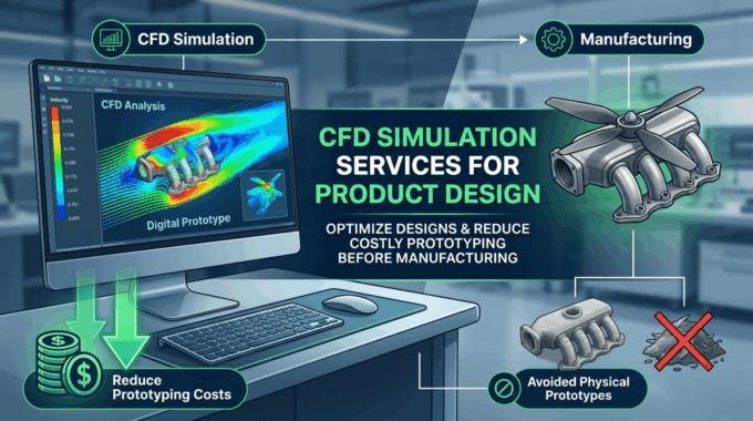
CFD Simulation Services for Product Design: Reduce Prototyping Cost Before Manufacturing
In modern product development, the most expensive mistakes are often discovered after money has already…
Comments (0)