Meat Drying Process Simulation Using VOF Model and Porous Media Approach
$360.00 $144.00 HPC
- The geometry represents the meat sample and surrounding air domain, discretized with a structured mesh of 58,800 elements to accurately capture heat and mass transfer gradients.
- The meat drying process was simulated using CFD to analyze heat and mass transfer during drying.
- The VOF model was applied to capture multiphase interactions between liquid water and vapor.
- The meat was modeled as a porous medium to represent internal moisture transport.
- Infrared heating and air convection were used as drying mechanisms under two operating cases.
- Results showed that higher heat flux and temperature enhanced drying efficiency and reduced moisture content.
To Order Your Project or benefit from a CFD consultation, contact our experts via email (info@mr-cfd.com), online support tab, or WhatsApp at +44 7443 197273.
There are some Free Products to check our service quality.
If you want the training video in another language instead of English, ask it via info@mr-cfd.com after you buy the product.
Description
CFD Simulation of Meat Drying Process Using Volume of Fluid Model and Porous Media Approach
Description
The project of meat drying, investigates the drying process of meat using infrared heating and convective air flow, modeled through computational fluid dynamics (CFD) simulation. The main objective is to analyze the temperature distribution, moisture reduction, and mass transfer behavior of the meat during the drying phase. The simulation employs a multiphase flow approach to capture the complex interactions between liquid water and water vapor as moisture evaporates from the meat surface. Two cases were simulated to compare the effects of different air velocities, air temperatures, and heat generation rates on the drying performance. The study provides valuable insights into optimizing industrial meat drying processes, improving efficiency, and maintaining product quality. Another aim’s of this project is By using curve fitting, the results are estimated, based on the simulation results.
Geometry and Mesh
The simulation domain of meat drying, includes the meat sample and surrounding air region, designed to accurately represent the drying environment. The computational mesh consists of 58,800 elements, ensuring a balance between accuracy and computational cost. The mesh quality and resolution are chosen to capture steep gradients in temperature and moisture content near the meat surface, where phase change occurs. The geometry is structured such that the infrared heat source is applied 1 mm below the top surface of the meat, mimicking realistic heating conditions. The meat is modeled as a porous medium, which allows simultaneous heat and moisture transfer through conduction, convection, and evaporation processes
Model and Solver Settings
The numerical simulation of meat drying, employs the VOF (Volume of Fluid) model to handle the multiphase flow between water and vapor phases. The Standard k–ε turbulence model is used to predict turbulent flow characteristics in the air region. The infrared heating source is implemented volumetrically at 1 mm below the top surface, simulating the radiation absorption depth in real meat. A User-Defined Function (UDF) governs the mass transfer process, ensuring that phase change (evaporation) only occurs at the outer surface of the meat. Two simulation cases were considered:
| Case | Heat Source (kW/m³) | Air Temperature (°C) |
Air Velocity (m/s) |
| 1 | 724 | 30 |
2.5 |
| 2 | 2150 | 40 |
1.5 |
Case 1 of meat drying was run for approximately 410 seconds, and Case 2 for 1400 seconds, with additional curve fitting performed to predict long-term results at 18,000 s and 32,400 s. The solver settings ensured convergence in both thermal and mass transfer terms.
Results
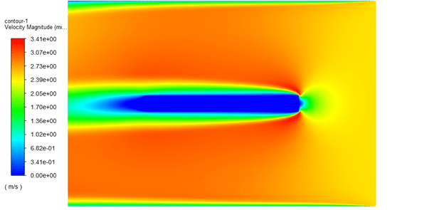
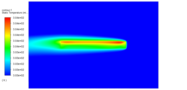
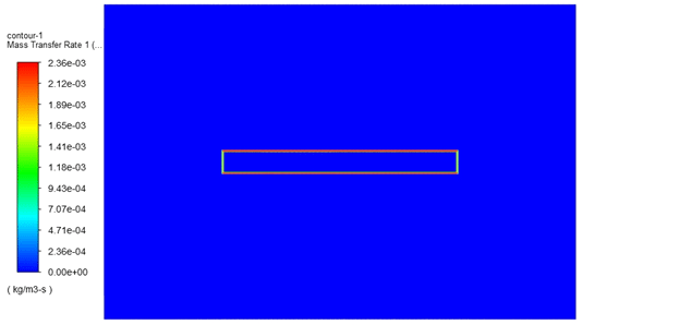
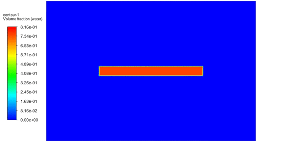
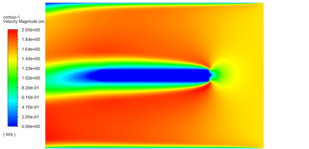
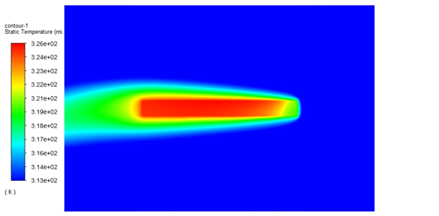
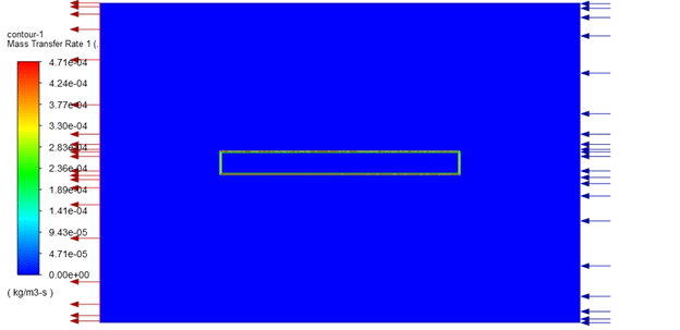
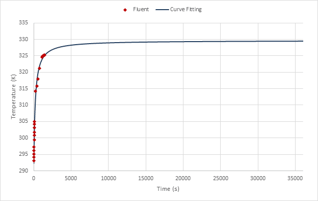
The results of meat drying reveal significant differences between the two cases of meat drying, due to variations in heat and flow parameters. In Case 2, with higher air temperature and stronger heat source, the meat temperature increased more rapidly, reaching about 329 K, compared to 307 K in Case 1. Moisture evaporation was faster in Case 2, with a lower final water volume fraction (~0.662) compared to Case 1 (~0.666). The velocity and temperature contours demonstrate enhanced convective heat transfer at higher temperatures, while the mass transfer rate plots confirm active evaporation zones concentrated near the heated surface.
The curve-fitted equations derived from simulation data describe the time-dependent changes in temperature and moisture. These functions enable long-term prediction of drying behavior beyond the simulated time. Overall, the analysis shows that increasing heat flux and air temperature improves drying efficiency, though excessive heating may risk surface hardening or uneven moisture removal.
Velocity contour at t=1070 s for case 1
Temperature contour at t=253 s for case 1
Mass transfer rate at t=253 s for case1
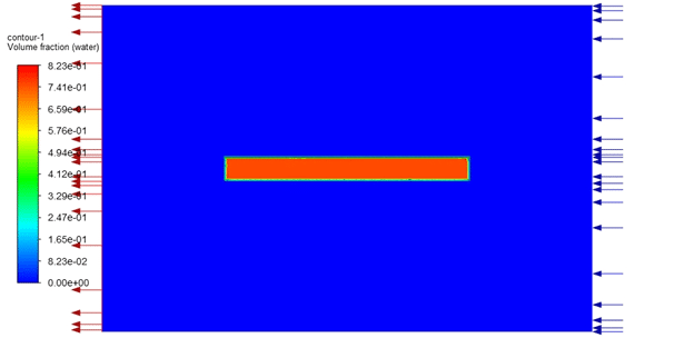
Water volume fraction at t=253 s for case 1
Velocity contour at t=1070 s for case 2
Temperature contour at t=1070 s for case 2
Mass transfer rate at t=1070 s for case 2
Water volume fraction at t=1070 s for case 2
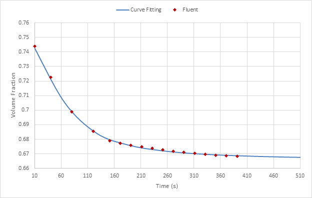
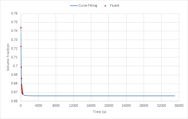
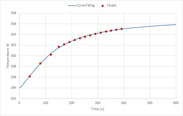
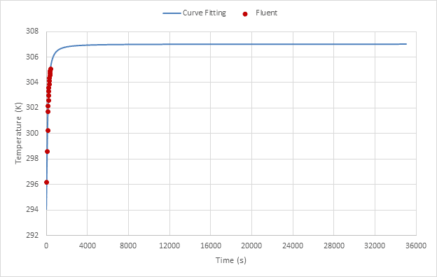
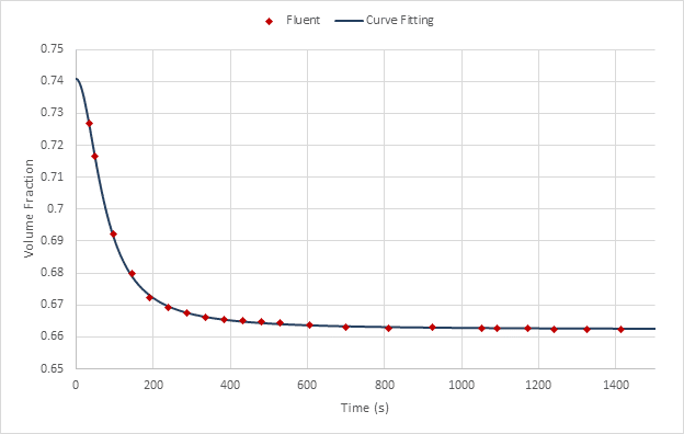
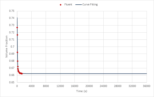
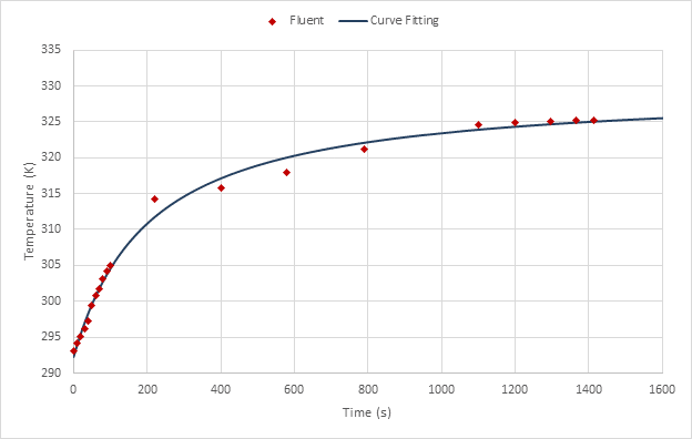
Case 1 and 2 were simulated about 410s and 1400s, respectively. By using curve fitting, the results are estimated. Based on the simulation results, a function in form of below was used to do curve fitting.
Case 1:
The coefficients of considered function for case 1 are represented in following table:
| Equation | a | b | c | d |
| Volume fraction | 0.7462049 | 1.816868 | 64.84147 | 0.6659228 |
| Temperature | 294.048 | 1.465865 | 122.3674 | 307.005 |
Case 1: Volume fraction
Case 1: Temperature
Case 1: Temperature
Case 2:
The coefficients of considered function for case 2 are represented in following table:
| Equation | a | b | c | d |
| Volume fraction | 0.7408438 | 1.942405 | 73.71991 | 0.6623425 |
| Temperature | 292.274 | 1.008927 | 203.0858 | 329.6682 |
Case 2: Temperature
Case 2: Temperature
By using curve fitting the results are calculated at 18000s and 32400s as follow:
| Case | Time (s) | Volume fraction | Temperature (K) |
| 1 | 18000 | 0.66592572 | 306.996394 |
| 32400 | 0.6659238 | 307.001363 | |
| 2 | 18000 | 0.66240731 | 329.2672014 |
| 32400 | 0.662406401 | 329.4455207 |
You must be logged in to post a review.


Reviews
There are no reviews yet.