Simulating Blade Flutter Using a Two-Way FSI Approach in Ansys: An Advanced Guide

In the high-stakes world of aerospace and turbomachinery R&D, few challenges are as notoriously difficult—or as critical—as predicting fsi blade flutter. We have all seen the catastrophic footage of the Tacoma Narrows Bridge; now, imagine that same aeroelastic instability occurring on a composite fan blade rotating at 10,000 RPM. The result is not just a failed test; it is the potential loss of an engine, a prototype, or worst of all, safety accreditation.

As a simulation engineer, moving from steady-state CFD to transient aeroelasticity is a quantum leap in complexity. It requires a mastery of fluid dynamics, structural mechanics, and the delicate synchronization between them. At MR CFD, we frequently guide clients through this transition, turning what looks like a “black box” of errors into a robust, repeatable workflow.

This guide is not a basic button-clicking tutorial. It is a Principal Engineer’s roadmap to setting up a high-fidelity, Two-way FSI coupling Ansys simulation. We will dissect the physics, the mesh strategy, and the solver settings required to accurately capture the onset of flutter.

---

Why is Predicting FSI Blade Flutter Critical for Turbomachinery Safety?

For modern turbomachinery, the push for efficiency has led to thinner, lighter, and more highly loaded blades. While these designs improve thrust-to-weight ratios, they significantly lower the structural stiffness, making the blades susceptible to Flow-induced vibration (FIV).

Standard steady-state CFD or even “1-way” FSI (mapping pressure to stress) is woefully inadequate here. A 1-way coupling assumes the structure is rigid enough that its deformation does not alter the flow field. However, in a flutter scenario, the blade’s deformation actively changes the angle of attack, which changes the aerodynamic load, which further deforms the blade. This feedback loop is the definition of aeroelasticity.

If this feedback loop creates negative aerodynamic damping, the blade will extract energy from the flow, leading to self-excited oscillations that grow exponentially until structural failure occurs. Predicting this boundary using high-fidelity URANS is the only way to ensure safety before cutting metal.

---

What are the Aeroelastic Mechanisms Behind Blade Flutter?

To simulate flutter, you must understand the war being waged between three physical forces: inertial forces, elastic forces, and aerodynamic forces.

In a stable system, the aerodynamic forces act as a damper. When the blade vibrates, the air resistance opposes the motion, dissipating energy. In a flutter scenario, the phase lag between the blade’s motion and the unsteady aerodynamic pressure shifts.

When setting up your solver, you are essentially asking Ansys to solve the equations of motion where the aerodynamic force is not a constant input, but a function of time and displacement. To capture this accurately, you must ensure your simulation correctly resolves the following parameters:

• Mass Matrix: The inertial resistance of the blade.
• Damping Matrix: The structural damping inherent in the material (often very low for metals/composites).
• Stiffness Matrix: The restorative force of the blade.
• Aerodynamic Force Vector: The time-dependent load calculated by Fluent.

If the work done by the aerodynamic forces on the blade over one cycle is positive, the system is unstable.

---

How Should You Prepare the Geometry and Mesh for 2-Way Coupling?

The success of a Two-way FSI coupling Ansys simulation is determined long before you click “Solve.” It begins with the mesh. Unlike static simulations, your mesh must survive deformation.

For the geometry, you must ensure a clean, watertight interface between the fluid and solid domains. While Ansys System Coupling can handle non-conformal mappings, best practice dictates that you maximize the overlap accuracy.

Fluid Domain Requirements:

• Boundary Layers: You need high-quality inflation layers (prisms) to capture the boundary layer separation, which often drives stall flutter.
• Refinement Zone: Create a localized density box around the blade tip where the displacement will be highest.

Structural Domain Requirements:

• Mesh Quality: Hexahedral elements are preferred for their superior convergence in transient structural dynamics.
• Interface: The face of the blade in the mechanical model must exactly match the “wall” boundary in Fluent to minimize interpolation errors during data transfer.

What are the Best Practices for Dynamic Mesh Update Methods?

The dreaded “Negative Cell Volume” error is the bane of every aeroelasticity engineer. This occurs when the node movement in the fluid domain causes a cell to twist inside out. To prevent this in Ansys Fluent, you must use a robust Dynamic Mesh strategy.

1. Diffusion Smoothing: This is your first line of defense. It treats the mesh like a spring system. Set the diffusion parameter based on “boundary distance.” This ensures that nodes far from the blade absorb the deformation, preserving the quality of the boundary layer cells near the blade surface.
2. Remeshing: For large amplitude flutter, smoothing alone will fail. You must enable local remeshing.
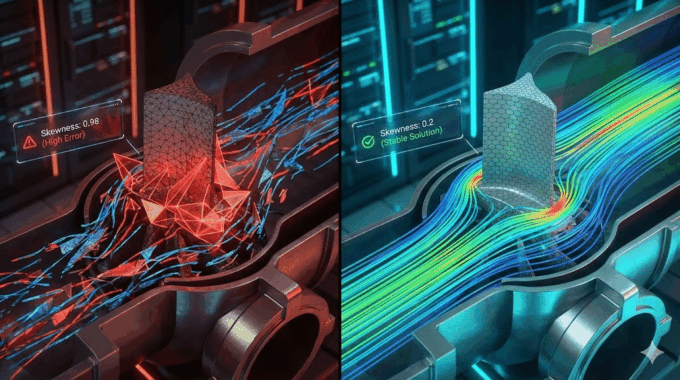
   • Pro Tip: Tightly control the “Maximum Skewness” and “Minimum Length Scale” criteria. If these are too loose, Fluent will generate poor-quality cells during the run, leading to divergence.
3. Layering: If the motion is purely linear (rare in blade flutter, which is usually modal), layering is efficient. However, for complex twisting modes, Smoothing + Remeshing is the standard Ansys System Coupling setup.

---

How Do You Configure the Transient Structural Analysis?

In Ansys Mechanical, you are not setting up a standard vibration test. You are setting up a Transient Structural analysis that accepts external pressure loads and returns deformation.

Crucially, you must account for the rotation of the machine. A static blade has different natural frequencies than a spinning one due to stress stiffening.

• Step 1: Run a Static Structural analysis with “Rotational Velocity” to establish the pre-stressed state.
• Step 2: Link this pre-stress condition to your Transient analysis.

Why is Modal Superposition Preferred over Full Transient?

You have two choices for the solver method: Full Direct Integration or Modal Superposition.

For fsi blade flutter, Modal Superposition is vastly superior in terms of computational efficiency.

• How it works: Instead of solving the full equations of motion for every degree of freedom (DOF) at every time step, the solver approximates the deformation as a weighted sum of the blade’s natural mode shapes.
• The Benefit: Since flutter usually excites only the first few modes (1st Bending, 1st Torsion), you can solve a massive model in a fraction of the time. This allows you to run longer simulations to see if the oscillation amplitude decays or diverges.

---

Which Ansys Fluent Settings Are Essential for Capturing Unsteady Aerodynamics?

To capture the phase lag that causes flutter, your CFD setup must be impeccable.

Turbulence Modeling:

Standard $k-\epsilon$ is often too dissipative and suppresses the flow separation that might trigger flutter.

• Recommendation: Use SST $k-\omega$ or, if computational resources allow, Scale-Adaptive Simulation (SAS). These models better capture the onset of separation and the wake dynamics essential for Turbomachinery CFD analysis.

Time Step Size:

This is the most critical parameter. If your time step is too large, you act as a numerical filter, artificially damping out the flutter.

• The Strategy: You must base your time step on the frequency of the mode you are investigating. You need to resolve the oscillation cycle with sufficient granularity. A general rule is to aim for a specific number of time steps per cycle of the dominant natural frequency (e.g., the first torsion mode).

Dynamic Mesh Zones:

Ensure the blade surface is set to “System Coupling” in the Dynamic Mesh zones. This tells Fluent, “Do not move this yourself; wait for instructions from Mechanical.”

---

How Do You Execute the Two-Way FSI Coupling in Ansys Workbench?

The Ansys System Coupling setup acts as the conductor of the orchestra, synchronizing Fluent and Mechanical.

1. The Schematic: In Workbench, drag the “System Coupling” component onto the canvas. Link the “Setup” cells of both Fluent and Transient Structural into the “Setup” of System Coupling.
2. Data Transfers: You need to define two distinct transfers:
   • Fluid Force $\to$ Structure: Fluent sends pressure and shear forces to the Mechanical blade surface.
   • Structural Displacement $\to$ Fluid: Mechanical sends the nodal deformations back to the Fluent wall boundaries.
3. Sequencing: The coupling service iterates within each time step.
   • Fluid solves $\to$ Forces transferred $\to$ Structure solves $\to$ Displacements transferred $\to$ Mesh updates.
   • This loop repeats until convergence is reached for that time step (defined by RMS convergence targets), then moves to the next time step.

---

How Do You Interpret Damping Ratios and Identify the Flutter Boundary?

Once the simulation is running, you will monitor the displacement of a monitor point (usually the blade tip) over time.

• Stable Response: You see an initial perturbation (perhaps from the startup impulse) that gradually decreases in amplitude. The Logarithmic Decrement is positive.
• Flutter (Unstable): The amplitude of oscillation grows with every cycle. The aerodynamic damping is negative.
• Limit Cycle Oscillation (LCO): The amplitude grows and then stabilizes at a high constant value due to non-linearities. This is also a failure mode.

To calculate the Aerodynamic damping ratio, you can post-process the displacement signal using the logarithmic decrement method on the peaks of the oscillation. This quantitative value is what you compare against your safety margins.

---

What Are Common Convergence Pitfalls in Strongly Coupled FSI?

Even for experienced engineers, Two-way FSI coupling Ansys simulations can be temperamental. Here are the most common issues we solve in our CFD Aerospace Consulting practice:

1. Under-Relaxation: If the fluid forces are high (e.g., water or high-pressure gas), the structural deformation can be violent, causing the fluid mesh to fail immediately.
   • Solution: Use a “System Coupling Under-Relaxation Factor” (e.g., 0.5 or 0.25) for the displacement transfer. This slows down the update speed, stabilizing the interaction.
2. Mesh Folding: This occurs when displacement is larger than the local cell size.
   • Solution: Improve the mesh stiffness coefficients in the Fluent Dynamic Mesh settings, or refine the remeshing parameters to trigger sooner.
3. Divergence in System Coupling: If the coupling iterations don’t converge, check your time step. It is likely too large for the structural response frequency.

---

Why Choose MR CFD for Your Next Aerospace R&D Project?

Simulating fsi blade flutter is one of the most resource-intensive and technically demanding tasks in engineering. It requires validating against experimental data, conducting Grid Convergence Index (GCI) studies, and managing massive data sets.

Internal engineering teams often struggle to allocate the dedicated time and HPC resources required to develop this workflow from scratch.

At MR CFD, we specialize in these high-fidelity simulations. Whether you need a turnkey consulting solution to validate a new blade design or an Ansys Fluent Advanced Course to upskill your team on Reduced Order Model (ROM) for flutter, we bridge the gap between academic theory and industrial application.

Don’t let convergence issues stall your product launch. Contact us today to discuss your aeroelastic challenges.

Frequently Asked Questions

What is the difference between 1-Way and 2-Way FSI for blade flutter?

One-way FSI is a unidirectional transfer: you run a CFD simulation, export the pressure loads, and map them onto a structure to calculate stress. It assumes the structure is stiff and does not affect the flow. Two-way FSI creates a feedback loop. As the blade deforms, it changes the flow path, shock position, and pressure distribution, which subsequently changes the deformation. For flutter prediction, 2-Way FSI is strictly required because flutter is an instability driven by this interaction.

How do I calculate the correct time step size for a flutter simulation?

The time step must be small enough to resolve the highest frequency mode of interest (usually the first torsional or bending mode). A widely accepted best practice is to use between 20 to 40 time steps per cycle of the dominant natural frequency. For example, if your blade’s natural frequency is 100 Hz (Period = 0.01s), your time step should be roughly $0.01 / 20 = 0.0005$ seconds. Using a larger time step will numerically dampen the result, potentially giving a false “stable” prediction.

Can I use the Energy Method instead of full 2-Way FSI?

Yes, the Energy Method is a common, computationally cheaper alternative. In this method, you prescribe the blade motion (based on a mode shape) in the CFD solver and calculate the work done by the aerodynamic forces on the blade over one cycle. If the work is positive, the flow is adding energy (unstable). However, the Energy Method assumes the vibration mode shape does not change due to the flow. Full Two-way FSI coupling Ansys is superior when non-linearities or mode-coupling are expected.

How do I prevent negative cell volume errors in Ansys Fluent during FSI?

Negative cell volume errors occur when the mesh motion distorts a cell beyond its geometric limits. To prevent this:

1. Ensure your initial mesh quality is high (low skewness).
2. Use “Diffusion” smoothing based on “Boundary Distance” with a diffusion parameter ($\alpha$) of 1.0 to 1.5.
3. For large deformations, enable “Remeshing” and set tight criteria for maximum skewness.
4. Decrease your time step size so the mesh moves less per increment.

What turbulence model is best for turbomachinery aeroelasticity?

For most industrial Turbomachinery CFD analysis involving flutter, the SST $k-\omega$ (Shear Stress Transport) model is the standard choice. It accurately handles the adverse pressure gradients and boundary layer separation that often trigger stall flutter. If you are investigating complex vortex shedding or deep stall flutter and have significant HPC resources, moving to Scale-Adaptive Simulation (SAS) or Detached Eddy Simulation (DES) will provide higher fidelity results by resolving the unsteady turbulent structures in the wake.