Discrete Phase Model (DPM): Boundary Conditions

Introduction

This article discusses DPM boundary conditions, including reflect, trap, escape, wall-jet and wall-film.

Discrete phase boundary condition

In discrete phase simulations, the interaction between particles and walls is essential to significantly predict a particle’s fate because wall impingement may cause a secondary breakup, splashing, leaving the domain, etc. It is handled by boundary conditions available in the Boundary Cond Type drop-down list under discrete phase model conditions shown in the figure.

Ansys Fluent gives us six options that will be discussed separately in the following.

Reflect Boundary Condition Type

The figure below shows that the particle rebounds after collision with the boundary. Thus, the momentum change is defined by the coefficient of restitution: (n: velocity in the normal direction to the wall, 2: represent velocity after collision, 1: represent velocity before the collision)

The tangential or normal coefficient of restitution varies between 0.0 and 1.0. The 1.0 value of the restitution coefficient implies that the particle retains its total momentum after the collision, either in a normal or tangential direction. Moreover, It is known as an elastic collision. On the other hand, if the coefficient of restitution equals 0.0, it means that the particle retains none of its momentum after the rebound.

Trap Boundary Condition Type

By applying the trap model to the DPM boundary condition type of a wall, the trajectory calculations are terminated after the collision, and the fate of the particle is counted as trapped. Furthermore, the entire mass is converted to the vapor phase in a droplet evaporation simulation. Check the figure below.

Escape Boundary Condition Type

If the DPM boundary condition type is set to escape the model, the particle vanishes after it encounters the boundary. Ansys Fluent sets the inlet’s and outlet’s DPM boundary conditions to escape type by default.

Wall-jet Boundary Condition Type

Theoretically, the wall-jet model is based on the Naber-Reitz theory, which defines velocities and directions by resulting momentum flux in a non-viscous jet. It is used when the wall film isn’t of the essence or cannot be formed, like on hot walls.

Wall-film Boundary Condition Type

In many industrial applications, the film formation on the walls is an important part that needs to be taken into consideration. For instance, imagine corona particles injected by human cough and forming a wall film on chair and table surfaces. When DPM particles are used to model wall film, particles can form a thin film after impingement. The basic mechanism schematic is shown.

Human Cough Virus Particles in the Coffee Shop

There are Four probable scenarios depending on impact energy and wall temperature. The following equation is the definition of impact energy:

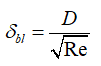
E: Impact energy, rho : liquid density, V_r : relative velocity of the particle in the frame of the impinging wall V_r²=(V_p-V_w)², D: droplet diameter, Sigma: surface tension of the liquid, h₀ :

current wall-film thickness,  : Boundary layer thickness 

The four scenarios mentioned before consist of Stick, Rebound, Spread and Splash. As depicted in the figure, below the boiling temperature of the liquid, the impinging droplet can eighter stick, spread, or splash. In contrast, the particles can rebound or splash above the boiling temperature. As a primary criterion, these values are estimated and can be used:

E<16: sticking

16<E<57.7: Spread

E>57.7: splashing

In summary, the particles join the film in the Stick regime, while in the Spread regime, particles join the film and move outward from the point of impingement. Above the boiling temperature and in the Rebound zone, particles bounce off the wall. At last, the Splashing mode has the most complex physics depicted.

Notes on wall-film model:

* The wall-jet model is more appropriate than wall film to model spraying on a hot wall. A thin vapor layer is assumed underneath the particles in the wall-jet model, so there is no direct contact between the particle and the boundary.

* In the wall-film model, the film thickness is very thin. It doesn’t exceed 500 microns, so the velocity field is considered a linear profile. The film particles are in direct contact with the boundary, which is totally different from the wall-jet model assumption.

* The film temperature never gets higher than the boiling temperature of the liquid.

* It is only available in transient simulations and may require small time steps.