CFD for Beginners Roadmap: 10 Essential Concepts You Must Know Before Starting CFD Learning

You’ve seen the stunning simulations—air gracefully flowing over a supercar, the intricate dance of combustion inside an engine, or the complex mixing of chemicals in a reactor.

You’ve wondered, “How do I create that?” For many aspiring engineers, Computational Fluid Dynamics (CFD) feels like a powerful but inaccessible field, guarded by complex mathematics and intimidating software. The sheer volume of information can be overwhelming, leading to a frustrating cycle of watching tutorials, clicking buttons, and getting nonsensical results. This is a common starting point, and it’s why a structured approach is not just helpful—it’s essential.

At MR CFD, with over 15 years of experience in both high-stakes industrial consulting and training thousands of engineers, we’ve seen firsthand what separates successful CFD practitioners from those who get stuck. It isn’t about memorizing every button in Ansys Fluent; it’s about mastering a core set of foundational concepts. This article is the clear, jargon-free CFD for beginners roadmap you’ve been looking for. We will break down the 10 essential pillars of knowledge that every successful CFD engineer builds upon. By the end, you won’t just understand the what; you’ll grasp the why, empowering you to move from a button-clicker to a confident engineering problem-solver.

Your Step-by-Step CFD Learning Roadmap

This table outlines a structured, four-phase path from absolute beginner to a competent CFD practitioner capable of tackling specialized problems. Follow this roadmap to build your skills logically and avoid common pitfalls.

Why Do You Need a Structured Roadmap to Learn CFD?

A common question we hear is, “Can’t I just jump into software tutorials on YouTube and figure it out?” While the enthusiasm is commendable, this approach often leads to a dead end. Random learning creates a dangerous illusion of competence. You might learn how to set up a specific case, but you won’t understand why you’re choosing a particular turbulence model, why your mesh quality is critical, or why your solution is diverging. This leads to unreliable, unvalidated results and a profound lack of confidence.

True CFD expertise is a knowledge pyramid. The base is a solid understanding of fluid dynamics physics. The next layer is the mathematics that describes that physics (like the Navier-Stokes equations). Only then comes the software (like Ansys Fluent) that implements the numerical solutions. The peak of the pyramid is the application—using the tool with sound engineering judgment to solve a real-world problem. Jumping straight to the software is like trying to build the pyramid from the top down; it will inevitably collapse.

What Happens When You Skip CFD Fundamentals?

Skipping the foundational concepts isn’t just inefficient; it’s a recipe for disaster. Here are three common nightmares we see from engineers who rushed the learning process:

1. Non-Converging Solutions: You set everything up, hit “Calculate,” and watch the residuals flatline or shoot to infinity. This is often caused by poor mesh quality or incorrect boundary conditions—fundamentals that were overlooked.
2. Physically Impossible Results: The simulation converges, but the results make no sense. A mechanical engineer once contacted our CFD consulting services after spending 72 hours on a simulation that showed fluid gaining energy as it passed through a simple pipe, a clear violation of conservation of mass and energy. The root cause? An incorrectly applied outlet boundary condition.
3. Wasted Computational Resources: Without understanding mesh independence, you might create a mesh with 20 million cells when 2 million would have given the same answer, wasting days of valuable computational time—a costly mistake, especially when using HPC for Ansys.

Understanding the fundamentals first saves you countless hours of frustration, builds true engineering intuition, and ensures your results can be trusted.

How Does MR CFD’s Beginner Roadmap Differ from Random YouTube Tutorials?

The internet is filled with scattered, context-free tutorials. Our approach is fundamentally different. The CFD for beginners roadmap embedded in our curriculum is built on a pedagogy of progressive complexity. We don’t just show you which buttons to click; we explain the engineering principles behind each choice.

• Structured Curriculum: Our CFD beginner courses are designed as a complete pathway, where each lesson builds logically on the last.
• Industry-Relevant Projects: You won’t be simulating flow over a 2D square. You’ll tackle projects that mirror real engineering challenges, from HVAC systems to automotive aerodynamics.
• Validation-Centric Methodology: Every project in our ANSYS Fluent training concludes with a critical step often missed in free tutorials: validating the simulation results against established experimental data or analytical solutions. This teaches the engineering rigor required for professional work.

We are a trusted learning partner because our methodology is proven to build confident, competent CFD engineers.

What is Computational Fluid Dynamics (CFD) and Why Does It Matter?

At its core, Computational Fluid Dynamics (CFD) is the science of using computers and numerical methods to predict how fluids—like air, water, oil, or blood—will behave. It allows us to simulate the flow, heat transfer, and chemical reactions of fluids in a virtual environment.

Its value proposition is simple and powerful: it allows engineers and scientists to test and optimize designs on a computer before building expensive physical prototypes. It’s like having a virtual wind tunnel, a virtual flow loop, and a virtual combustion chamber all on your desktop. This drastically reduces development costs, shortens design cycles, and enables innovation that would be impossible with physical testing alone.

What Real-World Problems Can You Solve with CFD?

CFD is not an academic exercise; it’s a critical tool used across nearly every industry to solve tangible problems. Here are just a few examples:

• Aerospace: Simulating airflow over an aircraft wing to maximize lift and minimize drag. (See our Aerodynamics/Aerospace Beginner Course)
• Automotive: Optimizing the cooling system of an engine or reducing the aerodynamic drag of a car to improve fuel efficiency.
• HVAC: Designing ventilation systems that ensure uniform air distribution and thermal comfort in a large office building. (Explore this in our HVAC Beginner Course)
• Biomedical: Simulating blood flow through a new stent design to predict its performance and minimize the risk of clotting. (Covered in our Biomedical Beginner Course)
• Energy: Designing more efficient heat exchangers for power plants or industrial processes. (Master this in our Heat Exchanger Beginner Course)
• Civil: Predicting wind loads on skyscrapers or modeling flood patterns in a river basin. (See applications in our Hydraulic and Civil Beginner Course)

How is CFD Different from Traditional Fluid Mechanics?

Classical fluid mechanics, which you study in university, provides exact, analytical solutions for relatively simple problems—like smooth, laminar flow in a perfectly straight pipe. These textbook solutions are invaluable for building intuition.

However, the real world is messy and complex. CFD tackles the problems classical methods can’t handle: turbulent flow, complex 3D geometries, and multiphysics interactions. Think of it this way: classical methods are like solving a puzzle with 10 pieces; CFD solves puzzles with 10 million pieces. CFD doesn’t replace theory; it extends its reach, allowing us to apply fundamental physical laws to problems of immense complexity.

Concept #1 – What Are the Navier-Stokes Equations and Why Are They the Heart of CFD?

You will inevitably hear about the Navier-Stokes equations, and they can sound intimidating. But don’t worry—you don’t need to solve them by hand. You just need to understand what they represent. In essence, the Navier-Stokes equations are the mathematical embodiment of the three most fundamental conservation laws of physics, applied to fluid flow. They are the heart of CFD because every fluid simulation, from air over a wing to water in a pipe, is an attempt to solve them.

What Physical Principles Do the Navier-Stokes Equations Represent?

Let’s break them down conceptually, without the scary math:

1. Conservation of Mass (Continuity Equation): This simply states that mass cannot be created or destroyed. For a fluid, it means “what goes in must come out,” unless there’s a source or sink. The amount of fluid entering a defined volume must equal the amount leaving it, plus any accumulation inside.
2. Conservation of Momentum (Newton’s Second Law): This is $F=ma$ applied to a fluid. It says that the rate of change of a fluid’s momentum is equal to the sum of the forces acting on it (like pressure forces and viscous forces).
3. Conservation of Energy (First Law of Thermodynamics): This states that energy can neither be created nor destroyed, only transformed. In CFD, it accounts for heat transfer through conduction, convection, and the work done by pressure and viscous forces.

Analogy Time! 💡 Imagine a water balloon. The total amount of water inside is constant (mass conservation). If you squeeze one side (apply a force), the water bulges out on another side (momentum conservation). If the water is hot, it will gradually transfer heat to the balloon’s rubber skin and the surrounding air (energy conservation). The Navier-Stokes equations mathematically describe this entire process.

Why Can’t We Solve Navier-Stokes Equations by Hand for Real Problems?

The Navier-Stokes equations are a set of coupled, nonlinear partial differential equations. For all but the simplest cases, there is no known general analytical solution. In fact, proving the existence and smoothness of solutions is one of the seven Clay Mathematics Institute Millennium Prize problems, with a $1 million reward.

This is precisely why we need CFD. Since we can’t find an exact, continuous solution for complex engineering problems, we use computers to find an approximate numerical solution that is “good enough” for engineering purposes.

How Do CFD Solvers Actually Use These Equations?

CFD solvers don’t solve the continuous equations directly. Instead, they use a process called discretization. This involves breaking down the fluid domain into thousands or millions of small cells (the mesh) and converting the partial differential equations into a system of algebraic equations that can be solved at each cell.

Think of it like a “connect-the-dots” game. The solver calculates the pressure, velocity, and temperature at the center of each cell. Once it has solved for these values at every single “dot,” it connects them to give you the complete picture of the flow field. Ansys Fluent primarily uses the Finite Volume Method, a robust and widely-used discretization technique that ensures conservation laws are honored at the cell level.

This need for a mesh is the perfect segue into our next core concept.

Concept #2 – What is a Computational Mesh and Why is it Your Simulation’s Foundation?

A computational mesh (or grid) is the digital skeleton of your simulation. It’s the process of dividing your fluid domain—the space where the fluid flows—into thousands or millions of smaller, simpler shapes called cells or elements. The discretized Navier-Stokes equations are then solved in each of these cells. The quality and type of your mesh are arguably the most critical factors determining the accuracy, convergence, and speed of your simulation.

What Are the Different Types of Meshes and When Should You Use Each?

There are three main families of mesh types, each with its own strengths and weaknesses:

• Structured (Hexahedral): Consists of an organized, grid-like structure of six-sided cells (hexes). This is the most efficient and accurate type but is generally restricted to simple geometries like pipes, channels, or simple airfoils.
• Unstructured (Tetrahedral/Polyhedral): Uses flexible, four-sided tets or multi-sided poly cells. This is perfect for highly complex geometries like engine blocks, pump volutes, or automotive bodies, as it’s much easier to generate automatically.
• Hybrid: A combination of both. A common strategy is to use a structured mesh near walls where flow gradients are high (like the boundary layer) and an unstructured mesh in the bulk flow region to handle geometric complexity.

Pro Tip: For most beginners working on complex parts, a high-quality polyhedral or poly-hexcore mesh in Ansys Fluent offers a great balance between accuracy and ease of generation. Our Mechanical Beginner Course provides practical examples of advanced meshing strategies for real industrial components.

How Does Mesh Quality Affect Your CFD Results?

The shape and quality of your cells matter tremendously. Poor quality cells can lead to inaccurate results and, more often than not, cause your solver to diverge. Key metrics to watch are:

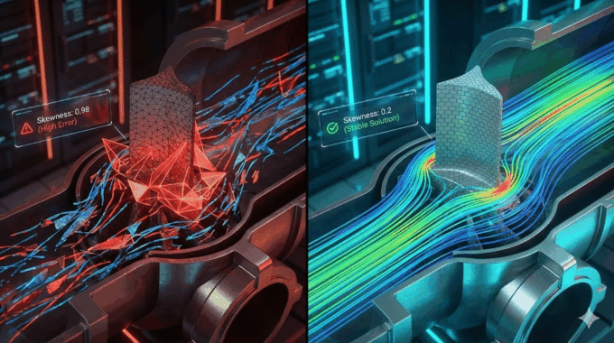
• Skewness: A measure of how distorted a cell is from its ideal shape (e.g., an equilateral triangle or a perfect cube). High skewness is a major cause of convergence problems. Rule of thumb: aim for a maximum skewness below 0.85.
• Aspect Ratio: The ratio of the longest to the shortest side of a cell. High aspect ratios are acceptable in one direction (e.g., in the boundary layer) but problematic if the cell is stretched in multiple directions.
• Orthogonality: A measure of how perpendicular the cell faces are to the lines connecting cell centers. Poor orthogonality can lead to numerical errors.

The golden rule of CFD is simple: Garbage mesh = garbage results.

What is Mesh Independence and Why Should You Care?

How do you know if your mesh is fine enough? The answer lies in performing a mesh independence study. This is a cornerstone of best practices in CFD simulation and demonstrates engineering rigor.

The process is straightforward:

1. Run your simulation on a relatively coarse mesh and record a key performance indicator (KPI), like the drag coefficient or the pressure drop.
2. Refine the mesh (e.g., by making the cells smaller) and run the simulation again.
3. Compare the KPI from the refined mesh to the coarse one.
4. Continue refining until the KPI stops changing significantly (e.g., less than a 1-2% change) between refinements.

At this point, you have achieved mesh independence. This ensures that your results are a property of the physics, not the mesh density. It prevents two common errors: under-refinement (inaccurate results) and over-refinement (wasted time and computational resources).

Concept #3 – What Are Boundary Conditions and How Do They Define Your Problem?

If the Navier-Stokes equations are the laws of physics and the mesh is the domain, then boundary conditions (BCs) are the rules of the game. They tell the solver what is happening at the edges of your computational domain—the inlets, outlets, and walls. Setting the correct boundary conditions is absolutely critical. Even with a perfect mesh and the right physics models, incorrect BCs will guarantee an incorrect solution.

What Are the Most Common Types of Boundary Conditions in CFD?

Here are five essential types you will use in almost every Ansys Fluent beginner tutorial:

• Velocity Inlet: Specifies the fluid velocity and properties at an inlet boundary. (e.g., “Air enters this duct at 10 m/s.”)
• Pressure Outlet: Defines the static pressure at an outlet boundary, allowing the flow to exit naturally. (e.g., “The exhaust exits to atmospheric pressure.”)
• Wall: Represents a solid boundary. The default is a “no-slip” condition, meaning the fluid velocity at the wall is zero relative to the wall. You also specify thermal conditions here (e.g., constant temperature or heat flux).
• Symmetry: Used to reduce the size of your computational domain when the geometry and flow are symmetric. This can save significant computational time.
• Periodic: Used for repeating patterns, such as the flow through a bank of tubes in a heat exchanger.

Analogy Time! 🏊 Think of a swimming pool. The jets where water enters are your inlets. The drains where water leaves are your outlets. The pool floor and sides are your walls. If the pool is perfectly still, the water’s surface can be a symmetry plane.

How Do You Choose the Right Boundary Conditions for Your Simulation?

Choosing the right BCs requires engineering judgment based on the real-world problem you are modeling. Follow this decision framework:

1. Know Your Physics: What are you trying to model? Is it forced convection driven by a fan (velocity inlet), or is it natural convection driven by buoyancy (pressure boundaries)?
2. Match Reality: Your BCs should reflect the actual operating conditions as closely as possible. What is the known flow rate? What is the downstream pressure?
3. Check for Compatibility: Some BC combinations are numerically unstable. For example, in an incompressible flow simulation, you should avoid setting a pressure inlet and a pressure outlet, as this doesn’t fix the mass flow rate and can lead to convergence issues.

Common Mistakes Box: ❌

• Specifying a velocity at an outlet (numerically unstable).
• Forgetting to apply thermal boundary conditions on walls in a heat transfer problem.
• Using a symmetry boundary when the flow itself is not symmetric (e.g., vortex shedding).

What Are Wall Functions and Why Do They Matter for Turbulent Flows?

Turbulent flow near a solid wall has extremely steep velocity gradients in a very thin region called the boundary layer. Fully resolving this with a mesh would require an enormous number of tiny cells, making many industrial simulations computationally prohibitive.

Wall functions are a clever solution. They are semi-empirical formulas that bridge the region between the wall and the fully turbulent core flow. Instead of resolving the boundary layer directly, they model its effect on the flow. This allows you to use a much coarser mesh near the wall, saving huge amounts of computational effort.

To use wall functions effectively, you need to be aware of the dimensionless wall distance, y+ (y-plus). For standard wall functions, the center of the first mesh cell off the wall should be in the log-law region, typically 30 < y+ < 300. Resolving the boundary layer directly requires a much finer mesh with y+ < 1. Our Heat Transfer Beginner Course includes hands-on exercises for calculating and achieving target y+ values.

Concept #4 – What is a CFD Solver and How Does it Calculate Flow Solutions?

The CFD solver is the engine that does the heavy lifting. After you’ve set up your mesh, physics, and boundary conditions, you click “Calculate.” The solver then begins an iterative process of solving the discretized algebraic equations for velocity, pressure, temperature, etc., in every single cell of your mesh. It repeats this process over and over, refining the solution with each iteration, until the results no longer change significantly.

What is the Difference Between Steady-State and Transient Solvers?

You’ll need to make a fundamental choice between a steady-state or transient simulation:

• Steady-State: This solver assumes that the flow properties do not change over time. It calculates the final, equilibrium state of the fluid flow. This is faster and computationally cheaper. Use it for problems like the constant airflow over a car at cruising speed or the pressure drop in a pipe at a constant flow rate.
• Transient (Unsteady): This solver captures how the flow changes with time. It solves the equations at discrete time steps. This is more computationally expensive but necessary for time-dependent phenomena. Use it for problems like the opening and closing of a valve, vortex shedding behind a cylinder, or the sloshing of fuel in a tank.

Pro Tip: If you care about when something happens, use a transient solver. If you only care about the final, stable state of what happens, use a steady-state solver.

What Are Pressure-Based vs. Density-Based Solvers?

Ansys Fluent offers two main families of solvers, each tailored for different flow regimes:

• Pressure-Based Solver: This was originally developed for low-speed, incompressible flows and is the workhorse for the vast majority of CFD applications (HVAC, hydrodynamics, many heat transfer problems). It solves the momentum and a pressure-correction equation in a segregated manner.
• Density-Based Solver: This was designed for high-speed, compressible flows where density changes are significant (supersonic flight, shockwaves). It solves the equations for continuity, momentum, energy, and species in a coupled set.

Rule of thumb: If the Mach number (the ratio of fluid velocity to the speed of sound) is less than 0.3, use the pressure-based solver. If Mach > 0.3, you should consider the density-based solver. Our Aerodynamics/Aerospace Beginner Course delves deep into the application of compressible flow solvers.

What Does “Convergence” Mean and How Do You Know Your Solution is Correct?

Convergence is the state where the iterative solution process has successfully reached a stable result. You monitor convergence by observing two things:

1. Residuals: These are indicators of the imbalance in the solved equations. As the solution progresses, the residuals should decrease. The goal is to drive them down by several orders of magnitude.
2. Monitored Quantities: These are key engineering values you care about, like drag, pressure drop, or mass flow rate. These values should stabilize and become flat as the solution converges.

Here are practical convergence criteria for most engineering simulations:

• Residuals drop below 10−3 for most variables, and below 10−6 for the energy equation.
• Key monitored values (like drag or pressure drop) change by less than 0.1% over the last 50-100 iterations.
• The overall mass and energy balance is conserved (imbalance < 1%).

Warning: Beware of “false convergence,” where residuals plateau at a high value. This usually indicates a problem with your mesh quality or setup. Remember, convergence does not equal accuracy. A converged solution can still be wrong if your setup is flawed. That’s why validation (Concept #9) is so important.

Concept #5 – What is Turbulence and Why is it the Biggest Challenge in CFD?

Most fluid flows you’ll encounter in the real world are not smooth and orderly (laminar); they are chaotic, swirling, and unpredictable. This is turbulence. From the wake behind a car to the flow from a faucet, turbulence is everywhere. It is often called the last great unsolved problem of classical physics because it is incredibly complex and computationally expensive to simulate directly. Therefore, for almost all industrial CFD, we rely on turbulence models.

What is the Difference Between Laminar and Turbulent Flow?

The key differentiator is the Reynolds number (Re), a dimensionless quantity that represents the ratio of inertial forces to viscous forces.

• Laminar Flow (Low Re): Viscous forces are dominant, leading to smooth, predictable, layered flow. Think of honey pouring from a jar or slow flow in a small pipe (typically Re < 2300).
• Turbulent Flow (High Re): Inertial forces are dominant, leading to chaotic eddies, vortices, and mixing. Think of river rapids or the air around a moving plane (typically Re > 4000).

Turbulence is crucial because it dramatically increases drag and pressure loss, but it also significantly enhances heat transfer and mixing—properties engineers must accurately predict.

What Are the Most Common Turbulence Models for Beginners?

Directly simulating all the chaotic swirls of turbulence (Direct Numerical Simulation or DNS) would require more computing power than exists in the world for most real problems. Instead, we use Reynolds-Averaged Navier-Stokes (RANS) models. These models don’t resolve the eddies; they model their average effect on the flow. The two most common RANS models for beginners are:

• k-ε (k-epsilon): This is the industry workhorse. It’s robust, computationally inexpensive, and good for free-stream flows away from walls. It’s a great starting point for many external aerodynamics or large-scale internal flow problems.
• k-ω (k-omega) SST: This model is generally more accurate near walls and is better at predicting flow separation due to adverse pressure gradients. It’s the preferred choice for applications like airfoils, turbomachinery, and many heat transfer problems where near-wall behavior is critical.

Simple Decision Tree: 🎯

• Is your flow external with potential for separation (like over a car or wing)? Start with k-ω SST.
• Is your flow a simple, fully developed internal flow? k-ε is often sufficient.

Advanced models like Large Eddy Simulation (LES) exist, but beginners should master RANS before attempting them.

How Do You Set Up Turbulence Parameters (Turbulent Intensity and Length Scale)?

RANS models need to know the approximate level of turbulence at the inlets of your domain. You provide this information using two main parameters:

• Turbulent Intensity (I): The ratio of the root-mean-square of the velocity fluctuations to the mean velocity. Typical values are 1% for low-turbulence wind tunnels, 5% for flows in pipes or ducts, and 10% for flows downstream of complex geometry.
• Turbulent Length Scale: A physical quantity related to the size of the largest eddies in the flow. A common estimate is about 7% of the characteristic length of your inlet (e.g., the pipe diameter).

The good news is that for most simulations, the results are not overly sensitive to these initial guesses (within a reasonable range). Don’t get stuck here; start with a reasonable estimate and proceed.

Concept #6 – What Are Material Properties and How Do They Influence Your Simulation?

A CFD simulation is only as good as its inputs, and a critical set of inputs are the physical properties of the fluid(s) you are modeling. These properties—like density, viscosity, and thermal conductivity—dictate how the fluid will respond to forces and temperature gradients. Using inaccurate properties will lead to inaccurate results, plain and simple.

What Are the Most Important Fluid Properties in CFD?

For most simulations, you will need to define these “big three” properties:

1. Density (ρ): The mass per unit volume (kg/m3). Density governs inertial effects (how much the fluid resists changes in motion) and buoyancy effects in natural convection. It can be defined as constant or as a function of temperature and/or pressure.
2. Viscosity (μ): A measure of a fluid’s resistance to flow or shearing ($Pa\cdot s$). A fluid with high viscosity is “thicker” (like honey) than one with low viscosity (like water). Viscosity is the source of wall friction and is critical for predicting pressure drop and boundary layer behavior.
3. Thermal Conductivity (k): The ability of a material to conduct heat ($W/m\cdot K$). This is essential for any simulation involving heat transfer.

For simulations involving the energy equation, you will also need the Specific Heat (Cp), which is the amount of energy required to raise the temperature of a unit mass of a substance by one degree.

When Should You Use Incompressible vs. Compressible Flow Assumptions?

This is a fundamental choice that depends on the Mach number (Ma), which is the ratio of the fluid’s speed to the speed of sound in that fluid.

• Incompressible Assumption (constant density): Use this when Ma < 0.3. This applies to almost all liquid flows and gas flows at low speeds (e.g., air flowing at less than 100 m/s or 225 mph). The solver assumes density is constant, which simplifies the equations and speeds up the solution.
• Compressible Assumption (variable density): Use this when Ma > 0.3 or when there are large changes in temperature or pressure that would significantly alter the fluid’s density. This requires activating the energy equation and is more computationally complex. Examples include high-speed aerodynamics, gas turbine combustion, and pipeline depressurization. Our Gas and Petrochemical Beginner Course covers compressible flow applications in detail.

How Do Temperature-Dependent Properties Affect Your Results?

For many problems, assuming constant material properties is acceptable. However, in simulations with large temperature variations (typically > 50-100 °C), this can lead to significant errors. The properties of most fluids, especially gases, change with temperature. For example, the viscosity of air nearly doubles between 0°C and 500°C.

In high-temperature applications like combustion, furnaces, or many heat exchangers, it is crucial to define material properties as a function of temperature (using polynomial fits or piecewise-linear profiles available in Ansys Fluent). Furthermore, all natural convection problems rely on the change in density with temperature (often simplified using the Boussinesq approximation) to create the buoyancy forces that drive the flow.

Concept #7 – What is Multiphase Flow and When Do You Need Special Models?

So far, we’ve mostly discussed single-phase flow—just one fluid, like water in a pipe or air over a wing. However, a huge number of real-world engineering problems involve the interaction of multiple phases of matter. These are multiphase flows, and they require specialized models beyond the standard CFD framework.

What Are the Main Types of Multiphase Flows in Engineering?

Multiphase flows are incredibly diverse and are typically categorized by the phases involved:

• Gas-Liquid: Examples include bubbles rising in a column, spray cooling, and ocean waves breaking. (See our Multi-Phase Flow Beginner Course)
• Liquid-Liquid: The separation of oil and water in the petrochemical industry or the creation of emulsions.
• Gas-Solid: The pneumatic conveying of powders, fluidized bed reactors, or the dispersion of pollutants from a smokestack. (Explore this in our DPM Beginner Course)
• Liquid-Solid: The transport of sand or slurry in a pipeline or sediment erosion in a river.

Modeling these flows is inherently more complex due to the need to track the interface between the phases and model the exchange of mass, momentum, and energy between them.

What is the VOF (Volume of Fluid) Model and When Should You Use It?

The Volume of Fluid (VOF) model is a surface-tracking technique designed for simulating two or more immiscible fluids where the position of the interface between them is important. In the VOF method, each cell in the mesh contains a variable representing the volume fraction of each phase. A cell with a volume fraction of 1 is full of that phase, 0 is empty, and a value between 0 and 1 contains the interface.

Use VOF for:

• Free-surface flows like dam breaks, ship hydrodynamics, or fuel sloshing in a tank.
• Stratified or layered flows, like oil and water in a separator.
• Tank filling and emptying processes.

Pro Tip: To get a sharp, well-defined interface, you need to use a fine mesh in the region where the interface is expected to be.

What is the DPM (Discrete Phase Model) and How Does it Differ from VOF?

The Discrete Phase Model (DPM), also known as a Lagrangian-Eulerian approach, is used for modeling dispersed flows where one phase consists of discrete particles, droplets, or bubbles suspended in a continuous fluid phase. Instead of tracking an interface, DPM calculates the trajectory of a large number of individual representative particles through the continuous fluid.

Use DPM for:

• Spray drying, paint spraying, or fuel injection in engines.
• Particle-laden flows where the volume fraction of the solid phase is low (typically < 10-12%).
• Soot formation, dust dispersion, or aerosol transport.

The key difference is the application: VOF is for large-scale interfaces, while DPM is for small, dispersed particles. Choosing the right multiphase model is one of the most critical decisions an engineer can make, as the wrong choice can lead to completely non-physical results. Our dedicated DPM Beginner Course provides a deep dive into setting up these simulations correctly.

Concept #8 – What is Heat Transfer in CFD and How Do You Model It?

Many, if not most, real-world CFD problems are not just about fluid flow; they also involve changes in temperature and the transfer of heat. To model these phenomena, you must activate the energy equation in your CFD solver. This allows you to simulate the three fundamental modes of heat transfer.

What Are the Three Modes of Heat Transfer in CFD Simulations?

Your CFD simulation can account for all three modes of heat transfer:

1. Conduction: Heat transfer through a solid or a stationary fluid, governed by Fourier’s Law. This is modeled automatically within both solid and fluid zones when the energy equation is active.
2. Convection: Heat transfer due to the motion of the fluid itself. This is the primary output of a thermal-fluid simulation, as it is directly captured by solving the flow and energy equations together. It can be forced convection (driven by a fan or pump) or natural convection (driven by buoyancy).
3. Radiation: Heat transfer via electromagnetic waves. This mode becomes significant at high temperatures (typically > 500°C) or in applications like furnaces, combustion, or solar loading. It requires activating a specialized radiation model in your solver, such as the P-1, Discrete Ordinates (DO), or Surface-to-Surface (S2S) model.

How Do You Set Up Conjugate Heat Transfer (CHT) Simulations?

Conjugate Heat Transfer (CHT) refers to the simulation of heat transfer that occurs simultaneously between solid and fluid domains. This is a very common industrial application—for example, analyzing the cooling of an electronics chip with a heat sink, or modeling the heat transfer from hot exhaust gas to the metal walls of a pipe.

Setting up a CHT simulation in Ansys Fluent involves:

• Defining both fluid and solid zones in your mesh.
• Assigning appropriate thermal properties (thermal conductivity, specific heat) to the solid materials.
• Ensuring that the interface between the solid and fluid zones is defined as a “coupled wall,” which allows the solver to automatically ensure continuity of temperature and heat flux across the boundary.

CHT is a powerful tool for thermal management, and it is a core topic in both our Heat Transfer Beginner Course and our specialized Heat Exchanger Beginner Course.

What Are Heat Transfer Coefficients and How Do You Extract Them from CFD?

The convective heat transfer coefficient (h) is a critical engineering parameter that quantifies the effectiveness of heat transfer by convection. Its units are W/m2⋅K. In simplified analysis, engineers often use empirical correlations to estimate an average h.

One of the great powers of CFD is its ability to calculate the local heat transfer coefficient all over a surface, providing much more detailed insight than a single averaged value. You can then:

• Create contour plots of h to identify areas of high or low cooling effectiveness.
• Calculate the surface-averaged h to get an overall performance metric.
• Use these CFD-derived values to validate against empirical correlations (often expressed using the dimensionless Nusselt number).

The heat transfer coefficient is calculated from the heat flux (q”), wall temperature (Twall​), and a reference fluid temperature (Tfluid​) using the formula: h=q“/(Twall​−Tfluid​). Reporting h correctly is a hallmark of a professional thermal analysis.

Concept #9 – What is Post-Processing and How Do You Extract Meaningful Results?

Running the simulation and achieving convergence is only half the battle. The real value of CFD lies in post-processing—the art and science of analyzing, visualizing, and interpreting the vast amount of data generated by the solver to extract meaningful engineering insights. A simulation without proper post-processing is just a collection of numbers.

What Are the Essential Visualization Techniques in CFD Post-Processing?

Good visualization tells a clear story about your flow physics. Mastering these five techniques is essential for any beginner:

1. Contour Plots: These are 2D color maps of a scalar quantity (like pressure, temperature, or velocity magnitude) displayed on a surface or a slice plane. They are perfect for quickly identifying hot spots, high-pressure zones, or areas of high velocity.
2. Vector Plots: These display arrows on a 2D plane, where the direction of the arrow shows the flow direction and its length/color represents the velocity magnitude. They are invaluable for understanding flow patterns and identifying recirculation zones or vortices.
3. Streamlines/Pathlines: These trace the path of imaginary, massless particles released into the flow field. They are one of the best ways to visualize complex 3D flow structures, mixing patterns, and trajectories.
4. Isosurfaces: These are 3D surfaces of a constant value. For example, you could create an isosurface of constant vorticity to identify the core of a vortex, or an isosurface of a specific temperature to visualize a flame front.
5. XY Plots: These are used for quantitative analysis, such as plotting the velocity profile along a line, plotting the pressure drop along the length of a pipe, or monitoring the convergence of a key value over iterations. They are crucial for validation against experimental data.

What Key Performance Indicators (KPIs) Should You Monitor in CFD?

Beyond pretty pictures, you need to extract hard numbers that define your design’s performance. These KPIs will depend on your application:

• Aerodynamics: Drag coefficient (CD​), lift coefficient (CL​), pressure drop.
• Heat Transfer: Average/maximum surface temperature, total heat transfer rate, average heat transfer coefficient, Nusselt number.
• Turbomachinery: Pressure ratio, efficiency, torque, mass flow rate.
• HVAC: Air change rate per hour (ACH), thermal comfort indices (PMV/PPD), velocity uniformity.

You should set up monitors in Ansys Fluent to track these critical KPIs during the solution process. This not only tells you when you’ve converged but also provides the final answer you’re looking for.

How Do You Validate Your CFD Results Against Experimental Data?

This is the most important step in the entire CFD workflow. Validation is the process of comparing your simulation results to reliable physical data (from experiments, analytical solutions, or peer-reviewed publications) to assess the accuracy of your model. Without validation, your simulation has no credibility.

The validation process follows an industry-validated CFD workflow:

1. Find Benchmark Data: Locate a published experiment or analytical solution for a similar problem.
2. Match Conditions: Set up your CFD simulation to match the geometry, boundary conditions, and material properties of the benchmark case as precisely as possible.
3. Compare Quantitatively: Compare your CFD results (e.g., from an XY plot) with the experimental data. Calculate the percentage difference or other error metrics.
4. Document and Explain: Document the comparison. If there are discrepancies, use your engineering judgment to explain potential sources of error, such as measurement uncertainty in the experiment or simplifying assumptions in your CFD model.

This rigorous process is a core tenet of our ANSYS Fluent training for beginners, ensuring you learn to produce results that can be trusted.

Concept #10 – What Are Solver Settings and How Do They Affect Convergence?

Beyond the physics models, there is a layer of numerical settings that can dramatically impact the stability, speed, and accuracy of your simulation. For beginners, it’s easy to leave these on their default values, but understanding what they do is key to troubleshooting convergence problems and ensuring your results are accurate.

What Are Discretization Schemes and How Do You Choose Them?

As we discussed, discretization schemes are the methods used to convert the continuous partial differential equations into algebraic equations. The “order” of the scheme relates to its accuracy.

• First-Order Upwind: This scheme is very stable and robust, making it great for starting a simulation or getting through difficult initial iterations. However, it is numerically diffusive, meaning it can smear out sharp gradients, leading to inaccurate results.
• Second-Order Upwind: This provides a much better balance of accuracy and stability and should be your goal for final results in most RANS simulations.
• Higher-Order Schemes (QUICK, MUSCL): These offer even higher accuracy but can be less stable and more prone to divergence. They are typically used for advanced applications like LES or DNS.

A typical professional workflow: Start the simulation with first-order schemes for the first 50-100 iterations to establish a stable flow field. Then, switch to second-order schemes to calculate the final, accurate solution. Never publish or report results based on a first-order scheme.

What Are Under-Relaxation Factors and When Should You Adjust Them?

Under-Relaxation Factors (URFs) are numbers between 0 and 1 that control the amount of change applied to a variable from one iteration to the next. Think of them as a “damping” or “stability” control. Lower values provide more stability but slow down convergence.

For 95% of cases, the default URFs in Ansys Fluent are well-tuned. However, if your solution is diverging or oscillating wildly, a common troubleshooting step is to reduce the URFs, particularly for pressure and momentum (e.g., reduce the pressure URF from 0.3 to 0.2). Conversely, if a simulation is very stable but converging slowly, you might be able to carefully increase the URFs to speed it up. Warning: Don’t just tweak URFs to fix a diverging solution; first, check for more fundamental problems like poor mesh quality or incorrect boundary conditions.

What Are Coupled vs. Segregated Solution Methods?

This refers to how the solver handles the pressure-velocity coupling in the Navier-Stokes equations:

• Segregated Algorithms (SIMPLE, SIMPLEC, PISO): These solve the momentum equations and the pressure-correction equation sequentially, one after another. They are memory-efficient and are the standard, robust choice for most steady-state problems. SIMPLE is the default and a great starting point for beginners.
• Coupled Algorithm: This solves the momentum and pressure equations simultaneously as a coupled system. It generally offers faster convergence, especially for complex physics like high-speed compressible flows or strongly buoyancy-driven flows, but it requires more memory.

Selection Advice: Start with the default segregated SIMPLE algorithm. If you have a good quality mesh and correct BCs, but convergence is still very slow, then you can try switching to the Coupled solver. Large coupled simulations often benefit from our CFD HPC services to handle the increased memory requirements.

How Do You Build a Practical Learning Path for CFD Mastery?

Now that you understand the 10 core concepts, how do you translate that knowledge into practical skill? The key is a structured learning path that builds complexity one step at a time.

What Should Your First CFD Project Be?

Don’t try to simulate a full F1 car on your first day. Start with a simple, well-documented, 2D benchmark case. This allows you to master the fundamental workflow without being overwhelmed by complex geometry or physics. Great first projects include:

• 2D Laminar or Turbulent Pipe Flow: This teaches you the entire workflow: basic meshing, setting inlet/outlet BCs, monitoring convergence, and, most importantly, validating your pressure drop results against the analytical solution or the Moody chart.
• 2D Flow Over a Cylinder: This introduces external aerodynamics, drag coefficient calculation, and can be extended to a transient simulation to visualize the famous von Kármán vortex street.
• 2D Natural Convection in a Square Cavity: A classic benchmark case for learning how to model buoyancy-driven flows and basic heat transfer.

Our Mechanical Beginner Course starts with these foundational projects to build your confidence on solid ground.

How Should You Progress from Beginner to Intermediate CFD Skills?

We recommend a three-stage progression, spending a few months on each stage with consistent practice:

1. Stage 1 (Beginner): Focus on mastering the end-to-end workflow for single-phase, steady-state simulations with simple physics. Complete 5-10 tutorial cases like the ones above. Your goal is to become comfortable with the software interface and the core concepts of meshing, BCs, and convergence.
2. Stage 2 (Intermediate): Start adding layers of complexity. Move on to 3D geometries, transient flows, heat transfer (including CHT), and basic turbulence modeling (k-ω SST). Tackle industry-relevant projects like a simple heat exchanger, airflow in an HVAC-equipped room, or the aerodynamics of a basic vehicle shape.
3. Stage 3 (Advanced): Now you are ready to explore the more complex physics models: multiphase flows (VOF, DPM), combustion, Fluid-Structure Interaction (FSI), advanced turbulence models (LES), and User-Defined Functions (UDFs).

MR CFD offers a complete curriculum with structured courses for each stage across a dozen different engineering disciplines, such as our popular courses for HVAC, Heat Exchanger, and Aerospace applications.

What Resources Does MR CFD Offer to Accelerate Your CFD Learning?

We have built a comprehensive learning ecosystem to support you at every step of your journey:

• Free Tutorials: Get started with our no-cost introductory projects to build confidence and experience our teaching style.
• Beginner Courses: Choose from over 12 discipline-specific learning paths, each providing 20-40 hours of hands-on, project-based training.
• Intermediate/Advanced Courses: Once you’ve mastered the basics, deepen your expertise in specialized topics like multiphase flow, combustion, or FSI.
• Consulting Services: If you get stuck on a real-world project or need expert results fast, our team of experienced engineers is here to help. (Learn more about MR CFD consulting services)
• HPC Services: For large, complex simulations, get access to our high-performance computing clusters on a pay-per-use basis. (Explore our MR CFD HPC services)

Our “learn by doing” philosophy is at the core of everything we do.

What Are the Most Common Mistakes Beginners Make in CFD?

Based on our 15+ years of teaching, we’ve identified a few common traps that beginners consistently fall into. Avoiding these will save you immense frustration and set you on the right path.

Why Do Beginners Often Trust CFD Results Without Validation?

This is the biggest and most dangerous mistake, often called the “pretty pictures syndrome.” A colorful contour plot looks authoritative and convincing, even if the underlying numbers are physically impossible. Beginners are often so relieved to get a converged solution that they forget to ask, “Is this solution correct?”

Blind trust is dangerous because:

• A poor mesh can show smooth contours but calculate the wrong forces or heat transfer rates.
• Using a laminar model for a turbulent flow will produce a completely wrong flow structure.
• Numerical errors from poor convergence can lead to non-physical results.

The Golden Rule: 📜 Never present or make an engineering decision based on CFD results that have not been validated against theory, experimental data, or at least a well-established benchmark case. Every project in our courses ends with a validation step to instill this critical habit.

What Happens When You Use Default Settings Without Understanding Them?

Ansys Fluent is a powerful tool with hundreds of settings. The defaults are designed to be robust and general-purpose, but they are rarely optimal for a specific problem. Relying on them blindly can lead to issues:

• Default Mesh Sizing: Often too coarse to capture critical flow features near walls or in areas with high gradients.
• Default Turbulence Model (often k-ε): Can be a poor choice for flows with strong separation or swirl.
• Default Discretization (sometimes first-order): Will produce overly diffusive and inaccurate results if not changed.

The goal is not to abandon defaults, but to make informed decisions. Understand what each key setting does, and then consciously choose to either keep the default or change it based on your problem’s physics.

How Do You Avoid the “Garbage In, Garbage Out” Trap?

The “Garbage In, Garbage Out” (GIGO) principle states that the quality of the output is determined by the quality of the input. CFD is a powerful amplifier of input errors. The three most critical inputs to get right are:

1. Geometry: Simplify your CAD model to remove small features (like bolts or logos) that don’t affect the main flow physics. But be careful not to over-simplify and remove a feature that is critical to the problem.
2. Boundary Conditions: These must reflect physical reality as closely as possible. If you are uncertain about a value (e.g., turbulence intensity), run a sensitivity study to see how much it affects your results.
3. Material Properties: Use accurate, reliable data for your fluids and solids. If properties are temperature-dependent, model them as such. Don’t guess.

Pre-Flight Checklist: ✅ Before you hit “Calculate,” always ask yourself: “Is my mesh quality acceptable? Are my boundary conditions physically realistic? Have I chosen the appropriate physics models for my problem?” This systematic check will prevent countless hours of wasted computational time.

How Can MR CFD Help You Master CFD from Beginner to Expert?

Choosing the right learning partner is the single most important decision you’ll make at the start of your CFD journey. MR CFD is dedicated to providing the most effective, industry-focused training available, designed to turn you into a confident and capable simulation engineer.

What Makes MR CFD’s Teaching Approach Different?

Our training methodology is built on five core principles that set us apart from academic lectures or random online tutorials:

• Industry-Focused Curriculum: Our projects are designed to solve real-world engineering challenges, not just simple academic “toy problems.”
• Progressive Learning: Our courses are carefully sequenced from fundamentals to advanced topics, ensuring you build a solid foundation without knowledge gaps.
• Hands-On Practice: You learn by doing. Every concept is reinforced with a guided simulation project, complete with downloadable files and step-by-step video instructions.
• Expert Instructors: You learn from practicing engineers with 15+ years of high-end CFD consulting experience, not just academics.
• Validation-Centric: We teach you to think like an engineer. Every project concludes by comparing results to experimental data, instilling the rigor needed for professional work.

Which MR CFD Beginner Course Should You Start With?

We offer over a dozen beginner courses tailored to specific engineering disciplines. Here’s a guide to help you choose:

• For a General Foundation: Start with the ANSYS Fluent Beginner Course. It covers the fundamental software skills applicable to all fields.
• For Mechanical/Automotive Engineers: The Mechanical Beginner Course is perfect, covering internal/external flows and heat transfer.
• For HVAC/Building Engineers: The HVAC Beginner Course focuses on room airflow, thermal comfort, and ventilation systems.
• For Aerospace Engineers: The Aerodynamics/Aerospace Beginner Course teaches airfoil analysis, drag/lift prediction, and compressible flow.
• For Biomedical Engineers: The Biomedical Beginner Course covers blood flow, stents, and respiratory simulations.
• For Thermal/Energy Engineers: Choose the Heat Transfer Beginner Course for fundamentals or the Heat Exchanger Beginner Course for a specific application focus.
• For Multiphase Applications: Start with the Multi-Phase Flow Beginner Course for VOF/Eulerian models or the DPM Beginner Course for particle tracking.

What Results Can You Expect After Completing MR CFD’s Beginner Courses?

After investing 30-50 hours to complete one of our beginner courses, you will have achieved:

• Technical Skills: The ability to independently set up, solve, and post-process common CFD problems in your field.
• Conceptual Understanding: You’ll be able to explain the why behind your choices, not just the how.
• Problem-Solving Ability: You will know how to diagnose common convergence issues and critically interpret your results.
• Career Impact: You will have a portfolio of validated, industry-relevant CFD projects to showcase to potential employers.
• Confidence: You will move from being intimidated by CFD to being competent and effective in its application.

What Are Your Next Steps to Start Your CFD Journey Today?

You have the roadmap. Now it’s time to take the first step. We offer multiple pathways to get started, catering to your readiness and goals.

How Can You Start Learning CFD Right Now for Free?

We believe in providing value upfront. You can begin your journey today with no cost or risk:

• Explore Our Free Tutorials: We offer a selection of free introductory projects to give you a taste of real-world CFD and our teaching style.
• Watch Sample Lectures: Preview content from our courses on our YouTube channel to see the depth and clarity of our instruction.
• Download Ansys Student Version: Get the free, full-featured Ansys Student software package, which is all you need for our beginner courses.

Which Paid Course Should You Invest In First?

Investing in a structured course is the fastest way to build job-ready skills.

• If you are a student or new to the field, start with the ANSYS Fluent Beginner Course for a comprehensive foundation.
• If you are a working engineer, choose the course specific to your discipline (e.g., Mechanical, HVAC, Aerospace) for immediate application to your job.
• If you have a specific thermal problem, the Heat Transfer Beginner Course is the perfect starting point.

All our courses come with lifetime access, downloadable project files, a certificate of completion, and instructor support.

How Can MR CFD’s Consulting and HPC Services Support Your Projects?

If you have an immediate, business-critical project, our professional services can deliver the results you need.

• CFD Consulting Services: Our team of expert engineers can take on your most complex simulation challenges, from initial setup to final reporting. This is ideal when you need guaranteed, validated results fast. Contact us for a custom quote.
• HPC Services: Don’t let computational limitations slow you down. Access our powerful high-performance computing clusters to run large, complex, or transient simulations on a flexible, pay-per-use basis. Learn more about our HPC offerings.

Frequently Asked Questions About Learning CFD

How long does it take to learn CFD as a beginner?

With consistent practice of 5-10 hours per week, you can become competent in setting up and running basic single-phase, steady-state simulations in about 3-6 months. A structured learning path, like one of MR CFD’s beginner courses, can significantly accelerate this process. However, CFD is a deep field; achieving true mastery is a career-long journey of continuous learning.

Do I need a strong background in mathematics to learn CFD?

While understanding the basics of calculus and differential equations is helpful for grasping the theory, it is not a strict prerequisite to become an effective CFD practitioner. Modern software like Ansys Fluent handles the complex math for you. More important are a strong intuition for physics, good engineering judgment, and a systematic, logical approach to problem-solving. Our courses focus on the practical application and conceptual understanding, not on deriving equations.

What computer specifications do I need for CFD simulations?

Here are some general guidelines:

• Beginner (Learning): A modern laptop or desktop with at least a 4-core CPU and 8-16 GB of RAM is sufficient for the tutorial-sized cases (under 512,000 cells) used in the free Ansys Student Version.
• Intermediate (Small Projects): A desktop workstation with a 6-8 core CPU and 32-64 GB of RAM is recommended for professional work on models up to 5 million cells.
• Advanced (Large Simulations): For models exceeding 5-10 million cells, or for complex physics like transient multiphase or LES, a workstation with 16+ cores and 128GB+ of RAM, or access to a High-Performance Computing (HPC) cluster, is necessary. Our MR CFD HPC services provide an affordable way to access this level of power.

Can I learn CFD without access to expensive software?

Absolutely. The Ansys Student Version is a free, full-featured version of the software that is perfect for learning. While it has a mesh limit (512k cells for fluids), this is more than enough to complete all the projects in any of our beginner courses. The skills you learn are directly transferable to the commercial version. Software cost should not be a barrier to starting your CFD journey.

What industries use CFD and what are the career opportunities?

CFD is used in virtually every major engineering sector:

• Aerospace & Defense
• Automotive
• Energy (Oil & Gas, Renewables, Power Generation)
• HVAC & Built Environment
• Biomedical & Healthcare
• Chemical & Process Industries
• Civil & Environmental Engineering
• Electronics Cooling

Job titles include CFD Engineer, Simulation Analyst, R&D Engineer, and Thermal Engineer. CFD is a high-demand skill, and professionals with this expertise often command higher salaries than generalist engineers. Our courses are designed to be career accelerators, giving you the practical skills employers are looking for.

How is CFD different from CAD, and do I need to know CAD first?

CAD (Computer-Aided Design) and CFD are two different but related tools in the engineering workflow.

• CAD is used to create the 3D geometry of a part or assembly. It defines the “what.”
• CFD is used to analyze the fluid flow and/or heat transfer within or around that geometry. It analyzes “how it performs.”

While basic CAD knowledge is helpful for creating or simplifying geometry, it is not a prerequisite to start learning CFD. Our courses provide all the necessary geometry files so you can focus on mastering the CFD workflow first.

What is the difference between CFD and FEA (Finite Element Analysis)?

Both are computer-aided engineering (CAE) simulation methods, but they analyze different types of physics:

• CFD is used for analyzing fluids (liquids and gases). It solves for things like velocity, pressure, temperature, and turbulence.
• FEA is used for analyzing solids. It solves for things like stress, strain, deformation, and vibration under structural loads.

The two fields overlap in multiphysics problems like Fluid-Structure Interaction (FSI), where the fluid pressure deforms a solid structure, which in turn changes the fluid flow. Here at MR CFD, we are experts in CFD and FSI.

Can I get a job as a CFD engineer after completing MR CFD’s beginner courses?

Our beginner courses provide the strong foundational skills that are a prerequisite for any junior CFD role. They demonstrate your initiative and capability to potential employers. While most dedicated CFD positions require an engineering degree and some project or internship experience, completing our courses will:

• Give you a significant advantage over other candidates.
• Provide you with a portfolio of validated, industry-relevant projects.
• Prepare you for the technical questions asked in interviews.

Many of our students have successfully used our courses to transition into CFD-focused roles or to add simulation skills to their existing engineering jobs.

How do I choose between MR CFD’s different beginner courses?

The best choice depends on your background and goals:

• Match your industry: The most direct path is to choose the course aligned with your field of study or work (e.g., an HVAC engineer should take the HVAC Beginner Course).
• Start broad: If you’re a student or unsure of your specialization, the ANSYS Fluent Beginner Course provides a universal foundation.
• Solve a problem: If you have a specific task, like designing a heat exchanger, choose that dedicated course (Heat Exchanger Beginner Course).

Remember, the core CFD skills are transferable. The fundamental workflow you learn in one course is applicable to all the others.

What ongoing support does MR CFD provide after I enroll in a course?

Our commitment to your success extends far beyond your initial enrollment. We provide a complete support ecosystem:

• Lifetime Course Access: Your learning never expires. Revisit lectures and projects anytime.
• Instructor Q&A: Get your questions about course content answered by our expert instructors.
• Community Forum: Connect with fellow learners to share insights and troubleshoot problems.
• Updated Content: Our courses are periodically updated to reflect new software versions and best practices.
• Certificate of Completion: A valuable credential to add to your resume and LinkedIn profile.

We are not just a course provider; we are your long-term partner in learning and mastering Computational Fluid Dynamics.