What is CFD Simulation (Computational Fluid Dynamics)? Comprehensive guide 2025
Computational Fluid Dynamics (CFD) has profoundly impacted how engineers and researchers approach fluid flow analysis, design optimization, and product development. It has given rise to sophisticated simulation platforms that enable experts to visualize and understand fluid behavior across a wide range of industries, from aerospace and automotive to biomedical and environmental engineering. In essence, What is Computational Fluid Dynamics simulation? It is an exciting field dedicated to simulating the movements of liquids and gases, revealing vital insights into physical phenomena that were once hidden behind costly experimental setups. Whether you’re an engineer in search of design optimization or a content creator aiming to share valuable information, Computational Fluid Dynamics (CFD) remains a transformative technology in modern engineering practices.
Over the years, the practical Benefits of CFD have grown exponentially thanks to advancements in computing power and software capabilities. Today, obtaining accurate simulation results is far more accessible, and the strategic use of CFD Services plays a crucial role in decision-making processes across various sectors. As a consulting engineering expert and content marketer for MR CFD, I’ve witnessed firsthand how improved simulation tools and best practices can help companies avoid costly prototypes, reduce time-to-market, and ensure the robustness of their products. These advantages have made CFD indispensable for any organization seeking to remain competitive in an ever-evolving technological landscape.
To delve deeper into the world of computational fluid dynamics, we will begin by breaking down the basics of CFD and explaining its place in modern engineering. Then, we’ll explore the leading simulation software, discuss critical governing equations, walk through typical project workflows, and even peek into the future of this dynamic field. By the end of this article, you’ll have a comprehensive understanding of What is CFD and how you can leverage its power to innovate and excel in your projects.
Concluding sentence: With that high-level overview in mind, let’s launch our journey into the realm of CFD by starting with a clear, concise demystification of this pivotal engineering discipline.
Before moving on to a deeper exploration of CFD, it’s essential to understand the core definition and objectives behind computational fluid dynamics so that the upcoming sections can be fully appreciated.
What is CFD Analysis?
Computational Fluid Dynamics (CFD) is a branch of fluid mechanics that uses numerical methods and algorithms to analyze and solve problems involving fluid flow, heat transfer, and related phenomena. Rather than relying solely on costly experimental setups or theoretical assumptions, CFD brings together mathematics, physics, and computational power to simulate real-world scenarios. By applying these simulations, engineers can predict how fluids—be they gases, liquids, or even multiphase mixtures—will behave under various operating conditions. In simpler terms, What is CFD Analysis? It’s a digital wind tunnel, water channel, or test bench that provides crucial data about flow characteristics long before physical prototypes are built.
From analyzing airflow over an aircraft wing to optimizing ventilation in indoor spaces, CFD enables the study of complex fluid behaviors. This could involve understanding turbulence patterns, boundary layer transitions, chemical reactions, heat exchange, and more. Its utility spans multiple disciplines: mechanical engineering, chemical engineering, biomedical engineering, environmental science, and beyond. The key advantage of CFD is its ability to offer insights into the Benefits of CFD—reducing trial-and-error and saving resources while improving accuracy and safety in designs.
Core Principles of CFD in Simple Terms
The fundamental principle driving CFD is the discretization of fluid flow equations, which transforms continuous physical phenomena into a set of algebraic equations solvable by computers. These equations, rooted in the Navier-Stokes equations, incorporate aspects of mass conservation, momentum conservation, and energy conservation. When applied to a discretized computational domain (a mesh or grid), they reveal velocity fields, pressure distributions, temperature gradients, and other vital parameters.
But how does CFD bring value in layperson’s terms? Think of it this way: if you want to know how a new car design might cut through air or how a pump might behave under varying inlet pressures, you can use a CFD model to emulate real-world conditions. This significantly cuts down on expensive prototyping. Moreover, software packages can present results in visually engaging formats—color-coded velocity contours, particle trace animations, and 3D renderings—making it easier for stakeholders to interpret the data and make informed decisions.
Concluding sentence: Having laid out the basics of Computational Fluid Dynamics, we can now shift our focus to the software tools that enable such detailed simulations, where programs like Ansys fluent and others take center stage.
Before we dive into the world of software packages, it’s worth appreciating how the field has evolved to offer numerous simulation platforms catering to different needs, budgets, and levels of expertise.
? Comprehensive Guide 2025 1")
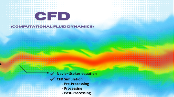
In general, and according to the figure above, the steps of solving a problem by computational fluid dynamics or CFD method are as follows:
- Pre-processing
- processing
- Post-processing
1. Pre-Processing
Pre-Processing is the first step in solving CFD analysis. The set of works done before entering the Fluent software (also other analysis software) and in Computer-Aided Design (CAD) environments such as design modeler, SpaceClaim, SolidWorks, CATIA, etc., and Meshing environments are the pre-processing stage.
In this step, we must do the following set of tasks:
- Create Geometry
- Create Mesh
- Physic Setting
- Select Solver
- Identify Models
- Identify Materials
- Specify Boundary Conditions
2. processing
After completing the Pre-Processing stage, we enter the next part, the processing or SOLVE stage. In this step, we do the following:
- Select Computing Algorithm
- Specify Discretization Method
- Specify Convergence Monitoring Criteria
3. Post-processing
Finally, you can view, Extract, and analyze the generated data and Results Checked, in the post-processing phase. Another name for this environment is CFD-Post or Result. At this point, the analyst can double-check the findings and develop conclusions based on them. Static or animated graphics, graphs, and tables are examples of ways to convey the results.
In summary, problem Identification (Define problem-solving goals, and specify the domain of the solution); We simulate specifying the geometry in the Computational Fluid Dynamics modeling procedure. Then discretize the geometry into a computational grid and incorporate into a computational domain (mesh). Physical, numerical models, beginning, and boundary conditions that characterize entirely the issue to be addressed must be set up to compute the problem’s solution.
It achieves the answer by executing the numerical method after the simulation setup. Finally, you extract them in the post-processing step the results.
Notice that the above steps should be repeated repeatedly, the results should be reviewed and analyzed, and each iteration in the Pre-Processing stage should be revised and corrected to achieve a citational answer.
? Comprehensive Guide 2025 2")
What is CFD Modeling
CFD Modeling or Computational Fluid Dynamics Modeling is all about harnessing numerical simulations to analyze and predict fluid flow behavior under specific conditions. In practical terms, CFD modeling transforms real-world fluid phenomena into data-driven insights by solving mathematical equations—essentially turning physical challenges into computational ones. As a result, engineers and researchers can visualize velocity fields, temperature gradients, and even chemical interactions without the immediate need for costly prototypes. This ability to simulate and optimize early in the design process stands among the core Benefits of CFD. Consulting firms like MR CFD offer specialized CFD Services to guide projects toward reliable and accurate results, while Ansys Training resources help new users get comfortable with powerful tools such as Ansys fluent (What is Ansys fluent?).
CFD Software Showdown: A Look at Leading Simulation Packages
In the realm of What is CFD, various software packages have emerged to cater to different industries and use cases. These tools range from free, open-source platforms to high-end commercial suites. The most popular choices typically include OpenFOAM, Ansys fluent, and COMSOL Multiphysics, each with its own set of pros and cons.
- OpenFOAM: As an open-source CFD toolkit, OpenFOAM is exceptionally flexible and popular among academia, research institutions, and industries looking for customizable solutions. Although its steep learning curve can be a hurdle, the upside is near-limitless adaptability. Development communities worldwide continuously contribute new solvers and libraries, making OpenFOAM a powerful choice for specialized simulations.
- ANSYS Fluent: Known for its user-friendly interface and robust solver capabilities, Ansys fluent stands out for industrial applications where reliability, extensive support, and comprehensive documentation are paramount. Users can dive into detailed multiphysics scenarios, advanced turbulence modeling, and fully coupled simulations. Because of its polished interface, it’s often the go-to solution for CFD Services in consultancy work. Ansys Training is widely available, making it easier for newcomers to get up to speed.
- COMSOL Multiphysics: Positioned as a multiphysics platform, COMSOL integrates CFD with other physical phenomena like structural mechanics and electromagnetics. This holistic approach is advantageous for projects that require tight coupling between different physics domains. However, some specialized CFD solvers might not be as advanced or as optimized as those found in dedicated CFD packages like Ansys fluent.
Pricing, Target Applications, and Ease-of-Use
Below is a comparative table summarizing key aspects of these popular CFD tools, including Pricing, Ease-of-Use, and Target Applications:
| Software | Pricing | Ease-of-Use | Target Applications |
| OpenFOAM | Free & open-source (requires investment in training/development) | Demands proficiency in scripting, command-line operations, and deeper theoretical knowledge; steep learning curve | Popular in academia & research labs focusing on code customization and advanced simulations |
| ANSYS Fluent | Commercial product (higher-end pricing, but includes support & updates) | Known for its intuitive GUI and guided workflow. Ideal for beginners, especially with Ansys Training resources available | Industry-focused projects requiring reliability, broad solver capabilities, and strong vendor support |
| COMSOL Multiphysics | Commercial product (cost scales with modules; can be expensive) | Integrated multiphysics environment; user-friendly for those familiar with COMSOL’s interface and approach | Scenarios demanding tight coupling between multiple physics (structural, EM, fluid, etc.) |
Pricing Considerations:- OpenFOAM stands out for being free, but organizations may need to invest in specialized training or dedicated developers to harness its full potential.
- ANSYS Fluent is generally on the higher end of the price spectrum but justified by its comprehensive features, professional support, and frequent updates.
- COMSOL can become costly if you require multiple modules for multifaceted simulations.
- Ease-of-Use:
- ANSYS Fluent provides a structured workflow, reducing the learning curve significantly.
- OpenFOAM, while powerful, requires a solid grasp of CFD theory and programming skills.
- COMSOL offers an integrated multiphysics environment, which can be user-friendly if you’re familiar with its interface.
- Target Applications:
- OpenFOAM is a favorite among organizations needing custom solvers and code-level modifications.
- ANSYS Fluent excels in industrial contexts where reliability, advanced turbulence modeling, and detailed support are critical.
- COMSOL is optimal when fluid flow is just one part of a broader multiphysics problem (structural, electromagnetic, etc.).
Concluding sentence: Armed with an overview of the leading software in the CFD realm, we’re now ready to explore the scientific foundation underlying these tools, namely the Navier-Stokes equations.
Before stepping into the realm of fundamental fluid mechanics, let’s see how these equations shape the robust capabilities of modern CFD solvers.
Beyond the Basics: Understanding the Navier-Stokes Equations in CFD
At the core of every CFD solver lie the Navier-Stokes equations, which govern the motion of fluid substances. These equations are derived from Newton’s second law of motion, but for fluids. They depict how momentum, mass, and energy are conserved within a fluid domain under various conditions. Rather than diving into heavy mathematical formulations, we can summarize them as follows:
- Continuity Equation: Ensures mass conservation, indicating that fluid cannot be spontaneously created or destroyed within the domain.
- Momentum Equations (Navier-Stokes): Describe how forces—such as pressure gradients, viscous stresses, and external accelerations—affect fluid motion.
- Energy Equation: Captures heat transfer, temperature distribution, and in some cases, phase changes or chemical reactions.
In CFD, these continuous partial differential equations are discretized into solvable algebraic equations. This is accomplished via methods like the Finite Volume Method (FVM), Finite Element Method (FEM), or Finite Difference Method (FDM). Software like Ansys fluent implements sophisticated numerical algorithms to solve these equations iteratively until a converged solution is reached.
Navier-Stokes equations
The final form of Navier Stocks equations is as follows:
? Comprehensive Guide 2025 3")
In these relations, u, v, and w show the velocities in the direction of x, y, and z, respectively.
Suppose these three momentum equations are combined with the Conservation of mass equation. In that case, they can give us a complete description of the different flow field properties of a Newtonian and incompressible fluid.
Due to the non-linear term in these equations, we cannot use an analytical solution, and we must approximate it numerically.
Role in Predicting Fluid Behavior
By applying the Navier-Stokes equations, engineers can predict velocities, pressures, and other crucial flow variables within a system. For example, in aerospace engineering, the equations guide the analysis of flow over airfoils, helping experts optimize lift-to-drag ratios. In the automotive sector, they aid in developing aerodynamic car shapes. In chemical and biomedical engineering, they help model mixing, blood flow, or heat exchange processes.
However, CFD is not just about plugging numbers into equations. It requires careful consideration of boundary conditions, fluid properties, and the nature of the flow (laminar or turbulent). The solutions can be incredibly accurate, but they also depend on how accurately the flow physics is captured, how appropriate the computational mesh is, and how well the solver settings are tuned. These complexities underscore the significance of robust simulation practices and, in many cases, guidance from seasoned professionals like MR CFD.
Concluding sentence: Having glimpsed the heart of the science behind CFD, we can now turn our attention to the crucial aspect of mesh generation, without which these equations could never be discretized accurately.
Moving forward, let’s discover why mesh quality can make or break a CFD project and how engineers strike the right balance between mesh resolution and computational resources.
Meshing Marvels: The Foundation of Accurate CFD Simulations
When exploring What is CFD Simulation, one quickly realizes that meshing is a critical step in the CFD workflow. The process of mesh generation involves dividing a geometric domain into smaller subdomains (elements or cells) over which the governing equations are solved. High-quality meshes capture the nuances of fluid behavior near boundaries, in regions of high curvature, and within zones prone to significant gradient changes (like boundary layers or shock waves).
Several mesh generation techniques are used:
- Structured Meshes: These have a regular, grid-like pattern. They can be efficient and lead to more straightforward solver algorithms, but they may struggle to conform to complex geometries without significant distortion.
- Unstructured Meshes: These typically feature triangles or tetrahedra (in 2D or 3D, respectively). They are far more flexible in capturing complex shapes and can be refined in local regions of interest. However, unstructured meshes might require more computational resources compared to structured ones.
- Hybrid Meshes: A combination of structured and unstructured elements (e.g., a boundary layer meshed with structured grids and the rest of the volume filled with unstructured elements). This approach can optimize both accuracy and computational efficiency.
Importance of Mesh Density and Trade-Offs
Mesh density plays a pivotal role in simulation accuracy. A finer mesh can capture more intricate flow details, such as turbulence vortices or sudden changes in temperature. However, it also leads to an exponential increase in computational cost and longer simulation times. Hence, engineers often perform a mesh independence study—running simulations with various mesh densities to find a suitable balance between result fidelity and computational feasibility.
Below is a simplified table outlining common trade-offs:
| Mesh Aspect | Impact on Accuracy | Impact on Computational Cost |
| Fine Mesh | Higher accuracy | Higher CPU/memory usage |
| Coarse Mesh | Lower accuracy | Lower CPU/memory usage |
| Adaptive Mesh Refinement (AMR) | Localized accuracy improvement | Dynamically increasing cost, but optimized |
Striking a balance often requires expertise. Tools like Ansys fluent offer sophisticated meshing modules that automatically refine regions of high gradient or curvature, minimizing user effort while maximizing solution quality. Having experts, such as MR CFD, review or develop your mesh strategy can significantly enhance the Benefits of CFD by ensuring reliable outcomes without overwhelming computational resources.
Concluding sentence: With a well-crafted mesh in place, we can now look at the real-world potential of CFD by examining its applications across a variety of industries.
Before we explore these examples, let’s see how meticulously designed meshes come to life in diverse sectors—from aerospace to environmental science—where CFD plays an indispensable role.
CFD Applications Across Industries: Real-World Examples in Action
One of the most impactful Benefits of CFD is its role in optimizing aerodynamic performance. In aerospace, CFD simulations help engineers refine wing designs, reduce drag, and improve fuel efficiency. By simulating airflow under various conditions, aerospace companies can predict lift and drag coefficients, enhance stability, and mitigate issues like flow separation. Meanwhile, in the automotive industry, CFD is employed to study the flow of air around vehicles, leading to refined shapes that reduce wind resistance and improve handling. Engineers also use CFD to enhance engine cooling, exhaust systems, and cabin ventilation—all without expensive wind-tunnel tests.
Case Study: Aerospace Wing Optimization
A prominent aircraft manufacturer leveraged CFD Services provided by MR CFD to optimize a commercial airliner’s wing design. Through parametric studies, advanced turbulence modeling, and repeated design iterations, the development team identified a wing shape that reduced drag by several percentage points. This translated into substantial fuel savings per flight, underscoring the Benefits of CFD in competitive industries.
Biomedical Engineering and Environmental Science
In biomedical engineering, CFD has revolutionized how researchers approach cardiovascular flow, respiratory system analysis, and medical device optimization. From artificial heart valves to stent designs, CFD simulations offer invaluable insights into how blood flows through intricate vessel geometries, guiding the design of safer and more effective devices.
Environmental engineers also tap into CFD to model pollutant dispersion, airflow in buildings, and natural ventilation strategies in urban planning. Through simulations of wind behavior and particulate matter transport, experts can propose better urban layouts and ventilation designs, safeguarding public health and reducing energy consumption.
Example: River Flood Modeling
Environmental scientists used CFD tools to simulate flood behavior in a river system with complex terrain. By predicting flow velocities, water levels, and possible inundation zones, they informed local authorities about crucial flood defense upgrades. This proactive measure helped communities better prepare for severe weather events, illustrating how CFD can support large-scale societal benefits.
Concluding sentence: As we can see, CFD permeates countless sectors, each benefiting from the technology’s ability to reveal deeper insights into fluid behavior, setting the stage for improved designs, safety, and innovation.
Next, we’ll break down the typical CFD project workflow—starting from conceptualization and geometry creation to final result interpretation—offering a roadmap for anyone looking to embark on a successful simulation journey.
From Concept to Simulation: A Step-by-Step CFD Workflow
1. Geometry Creation
The first phase of any CFD project involves generating or importing a geometry that accurately reflects the physical domain to be studied. Engineers use CAD (Computer-Aided Design) tools to produce a 3D model representing all the relevant features. A poor or oversimplified model can yield misleading simulation results, so meticulous design is essential at this stage. For complex designs, specialized software might be used to simplify geometry while preserving critical flow features.
2. Meshing
Once the geometry is ready, the next step is meshing, which we covered in detail in the previous section. A well-structured or carefully refined unstructured mesh ensures the accuracy of subsequent calculations. With software like Ansys fluent, automated tools can help identify complex regions—like small gaps or sharp edges—and refine the mesh accordingly.
3. Solver Setup
The solver setup phase includes defining:
- Physics Models: Whether the flow is laminar or turbulent, compressible or incompressible, single-phase or multiphase.
- Boundary Conditions: Speeds, pressures, and temperatures at inlets, outlets, walls, etc.
- Material Properties: Fluid density, viscosity, thermal conductivity, and other relevant properties.
- Solver Parameters: Numerical schemes, convergence criteria, and relaxation factors.
This step often demands expertise because picking the wrong model or boundary conditions can invalidate the results. Engineers sometimes rely on CFD Services from MR CFD to ensure correct setup—especially for complex or specialized flow problems.
4. Running the Simulation
After configuring the solver, the simulation is run. The software iteratively solves the discretized Navier-Stokes equations throughout the mesh, updating flow variables like velocity and pressure. Convergence monitoring is crucial—engineers watch residual levels, integrated quantities, and other checks to ensure the solution stabilizes and is not diverging.
5. Post-Processing and Visualization
Upon convergence, post-processing tools allow users to visualize and analyze the data. These can include:
- Contour Plots: Velocity, pressure, temperature fields.
- Vector or Streamline Plots: Illustrating flow patterns.
- Graphs and Reports: Summarizing performance indicators (e.g., lift-to-drag ratio, heat transfer rates).
- Particle Traces: Showing how fluid particles move through the domain.
6. Verification and Validation
Even with a converged solution, verification and validation steps are essential. Engineers compare simulation results against analytical solutions, experimental data, or benchmark cases to confirm reliability. We’ll delve deeper into this in the next section, but it’s worth noting that thorough validation ensures stakeholders can trust the outcomes of CFD simulations.
Concluding sentence: With a clear workflow in mind, let’s take a deeper look at how experts confirm the credibility of their simulation results, an essential factor for making confident, data-driven decisions.
Next, we’ll explore the importance of verification and validation and how these processes help ensure that our simulations stand on solid ground.
Validation and Verification: Ensuring Reliable CFD Results
In the world of CFD, establishing trust in your simulation results is non-negotiable. Validation and verification (V&V) constitute a systematic approach to confirming that the numerical solutions are both mathematically correct and physically sound. Verification answers the question, “Are we solving the equations right?” while validation asks, “Are we solving the right equations?” Combined, these processes act as the bedrock for reliable and defensible simulation outcomes.
Whether you’re optimizing a jet engine, designing a new HVAC system, or studying pollutant dispersion, stakeholders will need assurance that the computed results reflect reality. Without rigorous V&V, even the most visually impressive CFD animations can lead to erroneous conclusions and risky design decisions.
Methods and Best Practices
- Verification Techniques:
- Code Verification: Comparing numerical solutions to known analytical solutions or method-of-manufactured solutions.
- Grid Convergence Studies: Running the simulation with progressively finer meshes to confirm that solutions converge to a consistent value.
- Time-Step Sensitivity: For transient problems, ensuring that smaller time steps don’t significantly alter results.
- Validation Techniques:
- Experimental Correlation: Benchmarking simulation results against reliable experimental data (e.g., wind tunnel measurements, flow visualizations, or field tests).
- Physical Similarity: Checking the dimensionless parameters (like Reynolds number, Mach number) to confirm that simulation conditions match real-world scenarios.
- Comparative Approaches: Comparing results across different CFD solvers or turbulence models for consistency.
Adhering to these practices is integral to a professional CFD workflow. MR CFD, for instance, incorporates rigorous V&V protocols in its CFD Services, ensuring that clients receive not just pretty pictures but data-driven insights they can rely on for high-stakes decision-making.
Concluding sentence: Having covered how to ensure simulations remain trustworthy, our next step is to discuss how aspiring engineers or professionals can master CFD through various educational pathways and resources.
Looking ahead, let’s discover the vast opportunities for learning CFD, from online courses to formal university programs, and examine the career paths available in this thriving domain.
Mastering CFD: Educational Resources and Career Paths
Online Courses, Certifications, and University Programs
For those eager to learn What is CFD and become proficient in it, educational opportunities abound. You can begin by enrolling in foundational fluid mechanics courses offered by universities and online platforms. Once you grasp the basics, specialized cfd course delve deeper into numerical methods, turbulence modeling, and advanced solver techniques.
- Online Platforms: Websites like Coursera, edX, and Udemy offer comprehensive courses taught by industry experts and professors. These can range from introductory overviews to specialized modules focusing on turbulence or multiphase flows.
- Certifications: Organizations and software vendors often provide certificates that can bolster your resume. Ansys fluent course stands out as an example—completing an Ansys fluent certification can demonstrate hands-on competence in one of the industry’s leading CFD solvers.
- University Programs: Many engineering departments now include specialized CFD tracks or electives in their graduate-level curriculums. Master’s or Ph.D. programs often revolve around computational fluid mechanics, providing extensive research opportunities.
Career Prospects and Opportunities
As more industries recognize the Benefits of CFD, the demand for skilled professionals continues to grow. A career in CFD can lead you into roles such as:
- CFD Engineer: Employed in sectors like aerospace, automotive, or energy to optimize designs and troubleshoot fluid flow issues.
- Research Scientist: In academic or government labs, pushing the boundaries of CFD modeling and advanced turbulence simulations.
- Consultant: Offering CFD Services for clients across diverse fields, providing expert solutions without the need for in-house CFD teams.
- Software Developer: Crafting new features, solvers, or pre/post-processing tools for commercial or open-source CFD codes.
If you’re looking to strengthen your capabilities or transition into a specialized role, specialized consulting companies like MR CFD can provide hands-on training, mentorship, and real-world project experience. The learning curve can be steep, but with the right resources and perseverance, CFD practitioners often find fulfilling careers that blend technical challenge with impactful innovation.
Concluding sentence: With a flourishing skill set and a growing job market in your favor, your next step might be to look ahead at emerging trends and technologies that will shape the future of CFD.
Next, we’ll explore how machine learning, high-performance computing, and advancements in meshing techniques are poised to revolutionize the world of simulation in the coming years.
The Future of CFD: Emerging Trends and Technologies
One of the biggest trends shaping CFD is the rise of High-Performance Computing (HPC). As simulations become more complex—think large-scale atmospheric studies or intricate hypersonic vehicle analyses—the computational demands grow exponentially. HPC clusters and cloud-based solutions provide the processing power needed to run these massive simulations quickly. Many CFD Services are now offered through cloud-based platforms, enabling smaller companies to harness the benefits of HPC without making huge capital investments.
Machine Learning Integration
Another transformative frontier is the use of machine learning (ML) and artificial intelligence (AI) in CFD. ML algorithms can accelerate meshing, predict turbulence closure terms more accurately, and assist in parameter optimization—thereby slashing simulation times. Some research teams are even training neural networks to emulate parts of the Navier-Stokes equations, significantly reducing computational overhead. Although these methods are still under rigorous validation, the potential for game-changing speed-ups and new insights is undeniable.
Advancements in Meshing Techniques
Meshing has always been a bottleneck for many users. Emerging technologies like voxel-based meshing, adaptive mesh refinement (AMR), and geometry-aware meshing algorithms promise to reduce manual interventions and errors. Enhanced automation will not only streamline workflows but also push the boundaries of what’s computationally feasible. Coupled with HPC, these meshing innovations could lead to more widespread adoption of high-fidelity simulations like Large Eddy Simulation (LES) or Direct Numerical Simulation (DNS).
Speculative Future Directions
- Digital Twins: Entire industrial plants or aircraft fleets might be virtualized for continuous real-time monitoring and predictive maintenance, powered by CFD-enabled digital twins.
- Quantum Computing: Although still in its infancy, quantum computing may one day upend our understanding of computational physics, potentially solving complex flow equations with unprecedented speed.
- Full Multiphysics Integration: Tools will become increasingly interconnected, allowing fluid, structural, thermal, and electromagnetic phenomena to be solved in a single, coherent framework.
Concluding sentence: These innovations collectively hint at a bright horizon for CFD, where speed, accuracy, and versatility continue to evolve in tandem, empowering engineers to tackle increasingly intricate design challenges and pushing the boundaries of what’s possible in fluid mechanics.
By understanding What is CFD, leveraging the Benefits of CFD, and tapping into resources like MR CFD, businesses and individuals alike can turn theoretical models into actionable insights—shaping a future where simulation-driven design is the norm rather than the exception. Whether you’re an aspiring student or a seasoned professional, now is the perfect time to dive deeper into the world of CFD, make meaningful contributions, and help propel engineering innovation to new frontiers.
The power of CFD is yours to harness—seize the opportunity, elevate your skills, and let the flow of innovation guide your path forward.
Related Posts
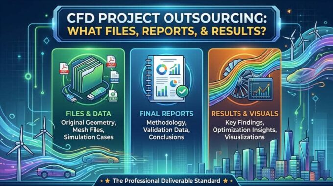
CFD Project Outsourcing: What Files, Reports, and Results Should You Expect?
When engineering teams decide to outsource CFD simulation, the conversation almost always starts with capability and…
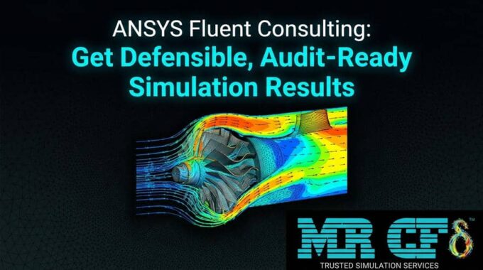
ANSYS Fluent Consulting: Get Defensible, Audit-Ready Simulation Results
You need ANSYS Fluent results that can survive scrutiny — a design review, a client…
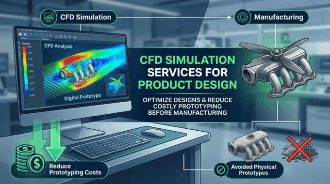
CFD Simulation Services for Product Design: Reduce Prototyping Cost Before Manufacturing
In modern product development, the most expensive mistakes are often discovered after money has already…
Comments (0)