
Finned Shell and Tube Heat Exchanger CFD simulation, ANSYS Fluent Training
$80.00 $8.00 Internship
The present problem simulates water flow and heat transfer inside a wavy-shaped finned shell and tube heat exchanger using ANSYS Fluent software.
Click on Add To Cart and obtain the Geometry file, Mesh file, and a Comprehensive ANSYS Fluent Training Video.To Order Your Project or benefit from a CFD consultation, contact our experts via email (info@mr-cfd.com), online support tab, or WhatsApp at +44 7443 197273.
There are some Free Products to check our service quality.
If you want the training video in another language instead of English, ask it via info@mr-cfd.com after you buy the product.
Description
shell and tube heat exchanger Project Description
The present problem simulates water flow and heat transfer inside a finned shell and tube heat exchanger using ANSYS Fluent software. The simulation model deals with a sample part of a heat exchanger. This section includes three computational areas for water flow; So that there is an area for upstream flow and one area for downstream flow and a middle area includes several tubes and fins. The water flow enters the computational zone with a velocity of 0.5 m.s-1 and a temperature of 343 K.
The fins merely act as a barrier or a kind of porous medium and have a thermal insulation boundary condition; While the tubes are assumed to have a constant temperature equivalent to 293 K on their walls.

Geometry & Mesh
The present model is designed in three dimensions using Design Modeler software. The geometry of the model is related to a part of the heat exchanger, the middle part of which has a sinusoidal or wavy structure and has several tubes and fins.

The meshing of the model has been done using ANSYS Meshing software and the mesh type is unstructured. The element number is 803864. The following figure shows the mesh.

shell and tube heat exchanger CFD Simulation
To simulate the present model, several assumptions are considered:
- We perform a pressure-based solver.
- The simulation is steady.
- The gravity effect on the fluid is ignored.
A summary of the defining steps of the problem and its solution is given in the following table:
| Models | ||
| Viscous | k-epsilon | |
| k-epsilon model | standard | |
| near-wall treatment | standard wall function | |
| Energy | On | |
| Boundary conditions | ||
| Inlet | Velocity Inlet | |
| velocity magnitude | 0.5 m.s-1 | |
| temperature | 343 K | |
| Outlet | Pressure Outlet | |
| gauge pressure | 0 pascal | |
| Wall – Tube | ||
| wall motion | stationary wall | |
| temperature | 293 K | |
| Wall – Fin | ||
| wall motion | stationary wall | |
| heat flux | 0 W.m-2 | |
| Methods | ||
| Pressure-velocity coupling | SIMPLE | |
| pressure | second order | |
| momentum | second order upwind | |
| turbulent kinetic energy | first order upwind | |
| turbulent dissipation rate | first order upwind | |
| energy | second order upwind | |
| Initialization | ||
| Initialization methods | standard | |
| gauge pressure | 0 pascal | |
| x-velocity | 0.5 m.s-1 | |
| y-velocity & z-velocity | 0 m.s-1 | |
| temperature | 343 K | |
Results
At the end of the solution process, two-dimensional and three-dimensional contours related to pressure, velocity and temperature, as well as velocity vectors and path lines are obtained.
Reviews
You must be logged in to post a review.
Mr. Walter Dach –
What an impressive level of detail in the simulation of water flow and heat transfer! The attention to the special construction of this finned shell and tube heat exchanger is commendable. It’s remarkable how accurately the thermal properties and flow dynamics are analyzed.
MR CFD Support –
Thank you for your kind words! We are very pleased to hear that you’re impressed by the level of detail and accuracy in the simulation. Our goal is always to provide high-quality and thorough CFD analyses. If you have any more questions about our products or if you need further assistance, feel free to reach out to us.
Christiana Koch –
I’m incredibly impressed with the meticulous detail and the results obtained from this simulation. It’s fascinating!
MR CFD Support –
Thank you so much for your kind words! We’re thrilled to hear that you’re impressed with the details and results of our Shell and Tube Heat Exchanger simulation. If you have any further interest in other simulations or need assistance with anything else, we’re always here to help!
Prof. Torrey Monahan –
Fantastic learning product! I was able to set up and simulate my finned shell and tube heat exchanger model with ease. The detailed boundary conditions and solver setup were explained brilliantly in the training, enabling me to comprehend the complex heat transfer interactions within the exchanger. It was fascinating to see the temperature distribution and fluid flow clearly with the provided contours. Kudos to MR CFD Company for developing such an insightful training module!
MR CFD Support –
Thank you for your review! We’re delighted to hear that you found our training for the ‘Finned Shell and Tube Heat Exchanger’ simulation in ANSYS Fluent helpful and insightful. It’s fantastic that you were able to visualize the temperature distribution and fluid flow effectively. We aim to deliver comprehensive learning experiences that resonate well with our users. Your feedback is highly appreciated, and it motivates us to keep providing high-quality CFD learning products. If you have any further queries or need more assistance, don’t hesitate to reach out!
Mortimer Nader –
I really enjoyed how this heat exchanger simulation captures the complexity of the design. It seems very robust and detailed. Learning from it has deepened my understanding of how finned heat exchangers work in practice!
MR CFD Support –
Thank you so much for your positive feedback! We’re delighted to hear that our simulation on the finned shell and tube heat exchanger using ANSYS Fluent was beneficial to you and heightened your understanding of heat exchanger mechanisms. Your enthusiasm for learning is exactly what we aim to inspire!
Ms. Marcella Spencer DDS –
I was really impressed with the way the fins were modeled as a porous medium with thermal insulation boundary conditions! The detailed setup steps in the table are extremely helpful to understand the simulation process.
MR CFD Support –
Thank you for your positive feedback! We’re glad you found the model setup and explanation clear and helpful. If you have any further questions or require more assistance in understanding our simulation processes, don’t hesitate to ask.
Carlos Keeling –
I appreciate the comprehensive nature of your CFD training product. Using ANSYS Fluent to simulate a shell and tube heat exchanger is extremely valuable, especially because it introduces concepts like boundary conditions, viscous models, and energy equations in a practical application. I believe this offers a blend of theoretic framework with hands-on experience that is indispensable for any engineer. Well done!
MR CFD Support –
Thank you for your positive feedback! We are thrilled to hear that you found the finned shell and tube heat exchanger simulation with ANSYS Fluent educational and valuable. It’s our goal to provide comprehensive training that combines theoretical concepts with practical application, and we’re glad that it’s making a difference in your understanding and learning experience. If you have any further questions or need additional support, feel free to reach out to us. Thank you for choosing MR CFD for your educational needs.
Mike Hammes Sr. –
This heat exchanger simulation with fins and tubes seems quite comprehensive! The layered detail in temperature, pressure, and velocity management, especially with assumptions like gravity neglect and thermal insulation boundary conditions, makes this appear to be a thorough and realistic study.
MR CFD Support –
Thank you for your positive feedback! We’re glad you appreciate the depth and comprehensiveness of our heat exchanger simulation training. Our goal is always to provide realistic scenarios and detailed studies to aid in understanding. If you have any more questions or need further assistance, feel free to reach out!
Dr. Meagan Hauck –
The simulation materials are comprehensive and helpful. The structured approach to applying boundary conditions and selecting appropriate models such as k-epsilon with standard wall functions indicates a thorough understanding of heat exchanger simulations. It’s great that the tutorial covers the initial setup details like velocity and temperature, which are essential for achieving realistic results. The inclusion of clear mesh images and methodical instructions for solver setup complement the tutorial well. I also appreciate the explanation of assumptions made, which helps in understanding the limitations and scope of the simulation. Excellent training for any CFD enthusiast or professional!
MR CFD Support –
We’re delighted to hear that our training materials on the Finned Shell and Tube Heat Exchanger simulation in ANSYS Fluent have met your expectations and proved so useful. Thank you for acknowledging the detailed setup and clarity of our instructions. It is our aim to provide comprehensive and user-friendly guides that assist our customers in achieving accurate simulations. Your thoughtful feedback is appreciated and motivates us to continue offering high-quality training resources.
Hassie Dach –
Very pleased with the level of detail in this course. The step by step simulation setup and outstanding visualization of the finned heat exchanger really helped me grasp the complex thermal processes involved.
MR CFD Support –
Thank you for your kind review! We’re thrilled to hear that our training material was able to shed light on the intricacies of heat exchange simulations. Your understanding and visualization of the complex processes are precisely what we aim for. If you ever have further inquiries or need assistance with similar projects, don’t hesitate to reach out to us!
Miss Thea Wisoky –
I’ve always been fascinated by how efficient heat exchangers can be! The complexity and precision that went into simulating a finned shell and tube heat exchanger in ANSYS Fluent truly showcase the capabilities of CFD to optimize industrial designs. Well done MR CFD Company.
MR CFD Support –
Thank you for your positive feedback! We’re thrilled to hear that our simulation has captured your interest in the efficiency of heat exchangers. It’s our goal to provide comprehensive and precise simulations to aid in understanding and optimizing designs. We appreciate your acknowledgment of the efforts put into this project.
Demond Hickle –
I was very impressed with the clarity of your simulation result presentation! Could you explain if the gravity effect was considered in your simulation and its potential impact on the performance of the heat exchanger?
MR CFD Support –
In this simulation for the finned shell and tube heat exchanger, gravity is ignored as mentioned in the simulation assumptions. This simplification is often made when the effect of buoyancy-driven flow is considered negligible compared to the forced convection effects, or when the flow direction minimizes the impact of gravity on the heat transfer and fluid flow. Eliminating the gravity effect could simplify the calculation and reduce computational resources without significantly impacting the validity of the results, given the flow and heat transfer conditions present in this scenario.
Athena Lang –
Fantastic learning product! The simulation seems comprehensive, and I appreciate the attention to detail in setting up the model particularly addressing the heat transfer and fluid flow intricacies in a finned shell and tube heat exchanger. Great balance between practical application and theory.
MR CFD Support –
We’re thrilled that our finned shell and tube heat exchanger simulation has met your expectations and has provided a detailed and practical learning experience. Your positive feedback is greatly appreciated, and we’re glad you found the balance between theory and application beneficial. Thank you for taking the time to review our product, and we hope it serves you well in your future simulations!
Oceane Weissnat –
The training for the Finned Shell and Tube Heat Exchanger CFD simulation was enlightening. Could you explain how the fins impact the heat transfer process within the heat exchanger?
MR CFD Support –
In the CFD simulation of the Finned Shell and Tube Heat Exchanger, the fins function as a barrier and a porous medium which facilitates increased surface area for heat transfer. Although they are set with a thermal insulation boundary condition for the sake of simplicity in this particular simulation, in reality, fins typically enhance the heat exchanger performance by improving the convective heat transfer between the tubes and the surrounding fluid.
Ewell Lemke –
This training material appears very comprehensive! The detailed step-by-step process, assuming no gravity effect in the model simplifies understanding the heat transfer within the heat exchanger. The constant temperature assumption for the tubes is helpful as a starting point for studying temperature distribution. Excellent resource for anyone interested in thermal simulations!
MR CFD Support –
We’re pleased to know that you found the training material comprehensive and helpful for understanding thermal simulations. Thank you for your positive feedback. Your satisfaction is our priority, and we look forward to providing you with more quality learning resources!
Miss Heloise Durgan III –
The course really shed light on the practical side of setting up and solving shell and tube heat exchanger simulations. Having hands-on examples and being able to follow along with a real project was beneficial. The step-by-step approach was easy to grasp and the explanations were clear. A really useful resource for anyone looking to polish their CFD skills in using ANSYS Fluent for heat transfer simulations.
MR CFD Support –
Thank you for the positive feedback! We are thrilled to hear that you found our shell and tube heat exchanger simulation course to be practical and understandable. Our goal is to provide comprehensive instructions that help users develop their skills efficiently. Your show of confidence is greatly appreciated, and we look forward to offering you more valuable learning experiences.
Prof. Faustino Fahey –
I am truly impressed by the thoroughness of the shell and tube heat exchanger simulation using ANSYS Fluent. Rarely do you see such detailed analysis and clear representation of flow characteristics within these systems. The inclusion of temperature differentials and water velocity on the fins and tubes captures the essence of heat exchanger operation succinctly. Great job on designing a simulation that not only educates but also practically informs design improvements.
MR CFD Support –
Thank you for your kind words and thoughtful feedback. It always brings us joy to hear when our customers appreciate the detail and effort we put into our simulation products. We are pleased to know that the simulation met your expectations and provided valuable insights. Your recognition means a great deal to us. Thank you once again for choosing MR CFD, and we hope our products continue to serve educational and practical purposes for you.
Glenda Lynch –
This training material seems extremely detailed and comprehensive, covering both geometry and setup. Can you explain if any special post-processing steps are included in the materials to help visualize and interpret the simulation results?
MR CFD Support –
Yes, the training material does include special post-processing steps. These ensure proper visualization and interpretation of the results. Those would typically cover how to generate two-dimensional and three-dimensional contours for parameters like pressure, velocity, and temperature, as well as how to visualize velocity vectors and path lines within the ANSYS Fluent software environment.
Alexa Schulist DDS –
I just wanted to share how impressed I am with the details provided in the ‘Finned Shell and Tube Heat Exchanger CFD simulation’ training! The setup sounds incredibly comprehensive, and it provides knowledge that bridges both academic theory and practical application. Understanding how to simulate complex heat exchange processes in ANSYS Fluent will undoubtedly be a major advantage in my engineering career. Great job on creating such a nuanced and technically rich learning experience!
MR CFD Support –
Thank you for recognizing the effort put into creating our ‘Finned Shell and Tube Heat Exchanger CFD Simulation’ training material. We strive to provide the most detailed and application-oriented learning experiences for our users, and it is rewarding to hear how beneficial you found it for your professional development. We’re thrilled to support you in your engineering journey and look forward to continuing to assist you with high-quality products!