Urban Housing Aerodynamics: A CFD Simulation

Description

Urban Housing Aerodynamics: A CFD Simulation of Airflow and Building Spacing Effects

Problem Description:

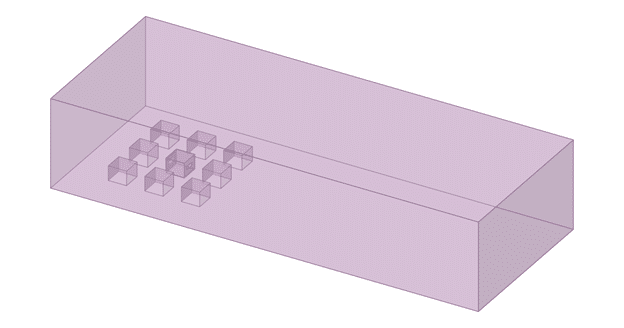
In the urban housing aerodynamics project, we study and numerically simulate the airflow entering a house located among eight other houses. For this purpose, we have selected a reference article titled “CFD analysis of cross-ventilation flow in a group of generic buildings: Comparison between steady RANS, LES and wind tunnel experiments”. The project’s primary goal is to investigate aerodynamics in three different cases. It is worth noting that the initial geometry (Figure 1) was taken from the article, which is one of the cases under study. We will discuss the geometry changes in detail below in the following steps. All simulations were performed using the ANSYS Fluent software.

Figure 1: Initial geometry extracted from the reference article

Geometry and Mesh:

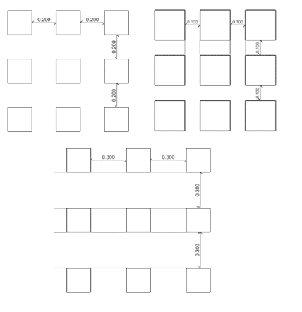
In the first step of the simulation of the urban housing aerodynamics project, the desired geometry was generated using the ANSYS SpaceClaim software. In the initial geometry extracted from the article, the distance between the two houses is 200 mm. In subsequent studies, this distance was changed to 100 mm in one case and 300 mm in the other. The general schematic of the house layout is shown in Figure 2.

Figure 2: General schematic of the layout of the houses in each case

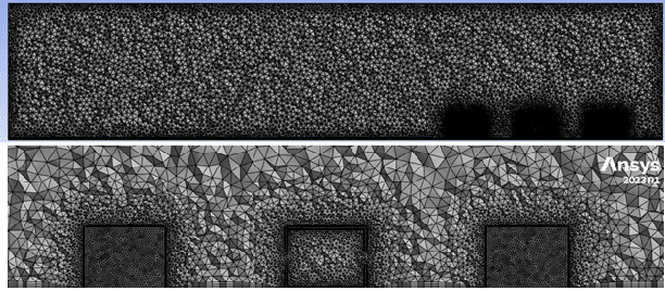
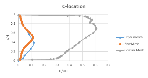
After creating the geometry of the urban housing aerodynamics project, the computational domain meshing was performed using ANSYS Machining software. Since the accuracy of the solution is of great importance, tetrahedral meshing was used in addition to the boundary layer mesh on all walls for this purpose. Two different mesh were generated and examined. In the first mesh, the element size was larger, which reduced the total number of computational cells, while in the second mesh, smaller elements were used for the urban housing aerodynamics project. The total number of elements in the second meshing is 5506508. The mesh quality is also high, considering the parameters of element elongation and orthogonality, so the average values ​​of these parameters ​​are reported to be 0.22 and 0.78, respectively. Also, the lowest orthogonality value is 0.2, and the highest element elongation value is 0.79. In Figure 3, a view of the cut domain is shown. It should be noted that comparing the results obtained from the two networks with the results of the paper indicates that the second network is better, and for this reason, it has been selected as the final network. Figure 4 shows the results of this comparison at the location of point C, which is the entrance to the central building.

Figure 3: Distribution of generated elements in the computational domain

Figure 4: Comparison of velocity profiles at position C for the first and second grids and the article

Setup:

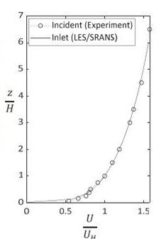
In the next step, we come to the main solver settings for the urban housing aerodynamics project. A pressure-based solver is used to solve the governing equations because the velocity in the domain is much lower than the level at which the fluid becomes compressible. The results are also extracted in steady state conditions. Finally, it is worth noting that the effects of the volumetric force of gravity on the fluid are considered. A standard two-equation k-epsilon turbulence model is used for the flow turbulence model. The boundary conditions of the problem are also defined according to the article. The side walls of the domain have the wall condition, and the symmetry condition is applied to the top wall. Also, the no-slip principle is considered on all walls. The critical point is the velocity in the inlet region, which is defined as the inlet velocity. Considering the velocity profile presented in the article, the velocity in the inlet region is not constant and is a function of the height above the ground. For this reason, a profile is used to model the velocity as in the article. Figure 5 shows the velocity profile in the inlet region.

Figure 5 – Velocity profile in the inlet area

The SIMPLE algorithm is used for the pressure -velocity coupling. The discretization of the governing equations is also performed with the upstream second-order model. It is worth noting that the pressure discretization is performed with PRESTO! to obtain results closer to the data of the paper.

To ensure the convergence of the urban housing solution, the residual values ​​are tracked up to the order of 10-5. In addition, the velocity in the exit region of the computational domain is controlled to achieve full convergence.

Results

First, it should be noted that the data presented in the paper generally have velocity profiles on a vertical line extending from the floor to the ceiling of the domain. Also, because all the sections are shown in one photo, it is impossible to find the velocity profiles accurately. A large part of the error is related to extracting the results from the paper. The data was collected in the form of point detection using Plot Digitizer software.

As mentioned earlier, the main goal of the urban housing research is to investigate the changes in the flow resulting from changes in the layout of the houses. Since the velocity gradient in each position can be different for each case, and it cannot be concluded which building has better ventilation, we will therefore consider the flow rate of the air entering the building. Given the definition of mass flow rate and the constant value of the inlet cross-sectional area and air density for all cases, the mass flow rate can be compared to the inlet velocity to the building in each case. The following table shows the mass flow rate reported in each case:

Table 1: Mass flow rate entering the building

According to the obtained data, it is observed that the mass flow rate entering the central building is higher in the case where the buildings are furthest apart. As the distance between the buildings decreases, the flow rate entering the building also decreases. Thus, considering the density and cross-sectional area being constant for all cases, it can be said that increasing the distance between the buildings increases the flow rate entering the central building. The reason for this is the pressure difference on both sides of the building because the pressure difference is the main factor for fluid flow. According to the results, the pressure difference on both sides of the building in case 1 is 1.69 Pascal, while this difference in case 3 is 3.3 Pascal. Figure 6 shows the pressure distribution along the fluid range in each case.

Figure 6: Pressure distribution in the middle plate for a) Mode 3, b) Mode 2, c) Mode 1

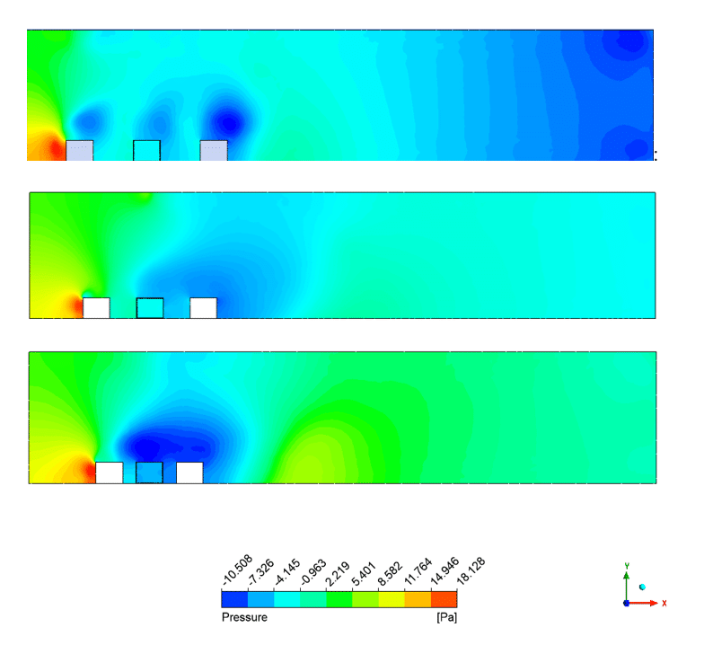
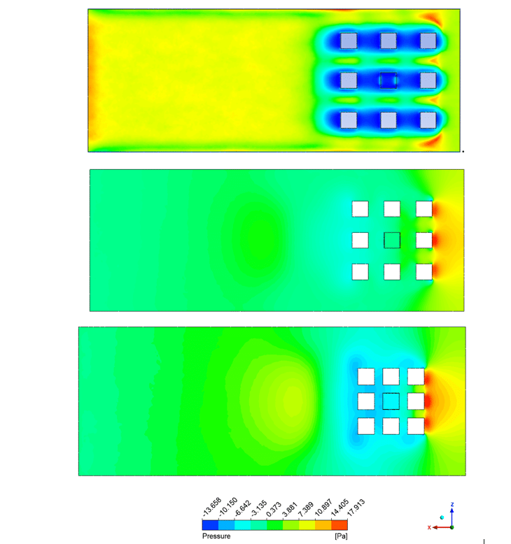
By examining the pressure distribution contours at a section at a height of 0.08 m, which is located in the middle of the entrance area of ​​the buildings, the effect of increasing or decreasing the distance between the buildings can be clearly seen. Figure 7 shows the pressure distribution in each case in the mentioned section.

Figure 7:  Pressure distribution in the cross section at a height of 0.08 m above the ground for a) Case 3, b) Case 2, c) Case 1

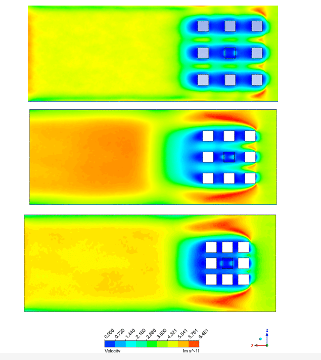
As can be seen, the flow creates a high-pressure area after entering the computational domain and colliding with the first-row buildings. It should be noted that the side walls of the fluid domain are modeled with the wall condition, so the fluid flow cannot escape from the side areas. An essential point in Figure 7 is the pressure value seen behind the buildings in case 3, i.e., the case where the distance between the buildings is 300 mm. Due to the considerable distance between the buildings, the fluid flow has a way to pass between the buildings, and this causes the high-pressure area not to be created, as in other cases. However, this area is very high-pressure when the distance between the buildings is 100 mm. The critical point is that these contours show the pressure distribution at a certain height, while by considering the entire fluid domain, the direction of fluid movement can be better predicted. For this purpose, the velocity contours are shown below (Figure 8). By observing the velocity distribution at this point, it is clear why ventilation is better as the distance between buildings increases.

Figure 8:  Velocity distribution