Forced Convection of a Non-Newtonian Nanofluid in Tube, Paper Numerical Validation
$270.00 $162.00 HPC
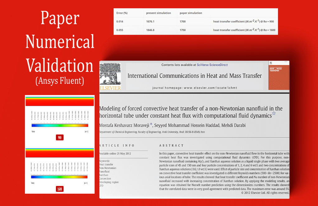
This simulation is based on the information of a reference article “Modeling of forced convective heat transfer of a non-Newtonian nanofluid in the horizontal tube under constant heat flux with computational fluid dynamics” and its results are compared and validated with the results in the article.
Click on Add To Cart and obtain the Geometry file, Mesh file, and a Comprehensive ANSYS Fluent Training Video.To Order Your Project or benefit from a CFD consultation, contact our experts via email (info@mr-cfd.com), online support tab, or WhatsApp at +44 7443 197273.
There are some Free Products to check our service quality.
If you want the training video in another language instead of English, ask it via info@mr-cfd.com after you buy the product.
Description
Paper Description
The present problem simulates the forced heat transfer of a non-Newtonian nanofluid in a horizontal tube using ANSYS Fluent software. This simulation is based on the information of a reference article “Modeling of forced convective heat transfer of a non-Newtonian nanofluid in the horizontal tube under constant heat flux with computational fluid dynamics” and its results are compared and validated with the results in the article. The nanofluid used in this model consists of water as the base fluid and xanthan and Al2O3 particles as its nano particles. The presence of xanthan causes the fluid to become non-Newtonian, and the presence of aluminum oxide particles causes the base fluid to become nanofluid.
The multiphase flow model is not used to define the nanofluid in this model; Rather, it is defined as a new material with thermophysical properties related to a nanofluid. Therefore, the current nanofluid inside the tube is defined with a density equal to 1126.384 kg.m-3 and a specific heat capacity equal to 3700.264 j.kg-1.K-1 and a thermal conductivity equal to 0.615 Wm-1.K-1. Be. Each of the values of the above thermophysical properties is obtained according to the relationships in the mentioned article. As mentioned, this nanofluid is a non-Newtonian fluid; So, it does not follow Newton’s law of fluids, and its viscosity changes with force.
Paper Description
Therefore, considering that the nanofluid flowing in the tube is a non-Newtonian fluid, the viscosity of the nanofluid is defined based on the herschel-bulkley model. According to the herschel-bulkley relationship, the values of the power-law coefficient and the yield stress threshold and the critical stress rate are 0.149, 2.92 pascal and 58.4 1.s-1, respectively. These coefficients are defined based on the data in Table 1 of the article. In this simulation, the nanofluid concentration is 4% and the nanofluid flow has two different Reynolds values (900 and 1600).
The following equation represents the value of the Reynolds number in terms of the value of the flow velocity in a non-Newtonian flow, the value of ƞ being defined in Table 1 of paper. So the value of the inlet flow velocity of the pipe is obtained according to this relation. This non-Newtonian nanofluid flows into the tube at a temperature of 295 K; So that the tube under constant heat flux is equal to 8846.4 W.m-2.
Geometry & Mesh
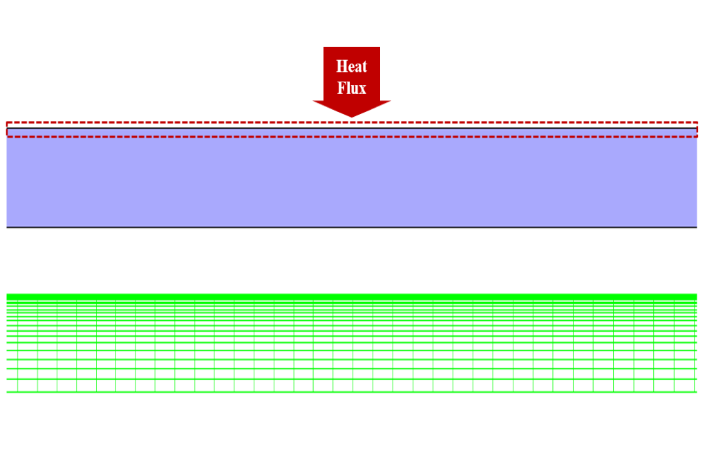
The present model is designed in two dimensions using Design Modeler software. This model includes a two-dimensional horizontal tube with a length of 1.2 m and a diameter of 0.00475 m. Since this model has a symmetric geometric, it is drawn as axisymmetric with cylindrical coordinates.
We carry out the meshing of the model using ANSYS Meshing software, and the mesh type is structured. The element number is 40000. The following figure shows the mesh.
Forced Convection CFD Simulation
We consider several assumptions to simulate the present model:
- We perform a pressure-based solver.
- The simulation is steady.
- The gravity effect on the fluid is ignored.
The following table represents a summary of the defining steps of the problem and its solution:
| Models (Forced Convection) |
||
| Viscous | Laminar | |
| Energy | On | |
| Boundary conditions (Forced Convection) |
||
| Inlet | Velocity Inlet | |
| velocity magnitude | 1.732714752 or 1.269787769 m.s-1 | |
| temperature | 295 K | |
| Outlet | Pressure Outlet | |
| gauge pressure | 0 pascal | |
| wall motion | stationary wall | |
| heat flux | 8846.4 W.m-2 | |
| Axis | Axis | |
| Methods (Forced Convection) |
||
| Pressure-Velocity Coupling | SIMPLE | |
| pressure | second order | |
| momentum | second order upwind | |
| energy | second order upwind | |
| Initialization (Forced Convection) |
||
| Initialization methods | Standard | |
| gauge pressure | 0 pascal | |
| axis-velocity | 1.732715 or 1.269788 m.s-1 | |
| temperature | 295 K | |
Paper Validation & Results of Forced Convection
The validation of the present simulation is based on the diagram in Figure 3-a of the mentioned article. This graph is related to the changes in the heat transfer coefficient of model (h) relative to the changes in the Reynolds number value. This diagram is for a state for which a dimensionless parameter defined in x/D form is equal to 147; So that parameter D indicates the size of the model diameter, which is equal to 0.00475 m. We perform the present simulation in two different values for the Reynolds number of 900 and 1600. The value of heat transfer coefficient is obtained according to the following equation (equation number 9 of the article).
Paper Validation & Results of Forced Convection
The amount of heat flux in this regard according to the data of the article is equal to 8846.4 W.m-2. Also Tw represents the wall temperature of the model and Tf represents the bulk temperature of the fluid. To obtain the value of these temperatures, we must create the resulting x value in the location (according to the above), a point on the model wall and a line passing through the model, respectively, and then we can obtain the values of the temperatures on them.
| Error (%) | present simulation | paper simulation | |
| 0.014 | 1676.1 | 1700 | heat transfer coefficient (W.m-2.K-1) @ Re = 900 |
| 0.055 | 1846.8 | 1750 | heat transfer coefficient (W.m-2.K-1) @ Re = 1600 |
At the end of the solution process, we obtain two-dimensional temperature and velocity counters in two different Reynolds values (900 and 1600). These contours are correspond to the middle part of the model.
Reviews
You must be logged in to post a review.



Alene Sipes –
How does the simulation account for the buoyancy effects induced by temperature differences within the storage container?
MR CFD Support –
The simulation accounts for buoyancy effects using the Boussinesq approximation, which is a common approach for modeling buoyancy-driven flows in CFD.
Pattie Murphy –
The review really appreciated the detailed analysis and adherence to the benchmark article’s parameters. Great work on demonstrating the validation process with numerical data!
MR CFD Support –
Thank you for your positive feedback! We strive to provide accurate and well-documented simulations, and it’s rewarding to hear that the efforts are appreciated. If you have any further questions or need more information on our simulation projects, feel free to reach out!
Letha Fritsch I –
I’ve observed some really good feedback from comparing the CFD results with those in the reference article. Considering the non-Newtonian characteristics and the nanofluid details are impressive. Does the inclusion of Al2O3 particles significantly enhance the thermal conductivity in the model compared to the base fluid alone?
MR CFD Support –
Thank you for your compliments on our comparison and detailed modeling with non-Newtonian nanofluids. In response to your question, yes, the inclusion of Al2O3 nanoparticles in the base fluid typically results in enhanced thermal conductivity. This is because nanoparticles have a high surface area to volume ratio, which facilitates better heat transfer, thereby increasing thermal conductivity compared to the base fluid alone.
Breanne Grady –
Fantastic course! The intricate details provided for the non-Newtonian nanofluid simulation were spectacular. Being able to follow along with a reference paper and validate results gave me immense confidence in my learning. Such clarity in the transition from academic theories to practical simulations in ANSYS Fluent is commendable.
MR CFD Support –
Thank you for your rave review! We’re thrilled to hear that our course on non-Newtonian nanofluid simulation met your expectations and helped you gain practical skills in ANSYS Fluent. Your success is what motivates us to provide clear, in-depth training. Keep up the fantastic work with your simulations!
Shakira Jenkins DDS –
How does the simulation handle turbulence near the walls of the storage container?
MR CFD Support –
The simulation uses wall functions to accurately model the turbulent boundary layer near the walls of the storage container.
Tremayne Pfannerstill –
Absolutely fantastic learning material! It matched the reference paper’s data, and it was incredibly rewarding to see the CFD concepts applied so accurately, especially the handling of the non-Newtonian nanofluids. The step-by-step approach clarified the entire simulation process from geometry creation to results validation. Loved the detailed explanation on defining viscosity using the Herschel-Bulkley model. Keep up the excellent work!
MR CFD Support –
Thank you for your kind words and for acknowledging the quality and detail of our material. We are thrilled to hear that our product helped deepen your understanding of non-Newtonian nanofluids and CFD methodologies. We always strive to provide clear, accurate, and practical learning resources. If you have any more feedback or need further assistance, don’t hesitate to reach out!
Jamir Gislason DDS –
Is there a possibility to see a comparison of the numerical results and those in the reference paper as part of the product documentation?
MR CFD Support –
Yes, the product documentation includes a comparison of the simulation results with the data from the reference paper to validate the simulation process. This comparison is presented in the form of graphs and tables, showing the effectiveness of the simulation process in predicting the heat transfer characteristics of the non-Newtonian nanofluid in the horizontal tube.
Andy Wolf –
I wasn’t completely sure about how the nanofluid properties, particularly the thermal conductivity, were determined. Could you explain a bit about how the inclusion of xanthan and Al2O3 nanoparticles affects the overall thermal conductivity reported for the nanofluid in the simulation?
MR CFD Support –
Certainly! The thermal conductivity reported for the nanofluid simulation includes the effects of both xanthan and Al2O3 nanoparticles. To calculate the effective thermal conductivity, it typically involves using different theoretical or empirical models that incorporate the conductive properties of both components and their volumetric proportions. In particular models, factors such as particle shape, size, distribution, and base fluid interaction are also considered. However, for specific methodologies like how the thermal conductivity was determined in this study, it would be best to reference the relationships and procedures detailed in the research article simulated here.
Mathilde Baumbach DVM –
What a thorough resource! It was so helpful seeing the principles of forced convection in non-Newtonian nanofluids brought to life. It’s fascinating how adding nanoparticles can change the properties of a fluid so dramatically. The use of the Herschel-Bulkley model for viscosity was an insightful choice.
MR CFD Support –
Thank you for your kind words! We’re pleased to hear that you found the simulation on the forced convection of non-Newtonian nanofluid insightful. Indeed, the complex behaviors exhibited by these fluids when nanoparticles are introduced make for a fascinating study, and applying the Herschel-Bulkley model allows for a more accurate representation of their rheological characteristics. Your appreciation truly motivates us to keep providing high-quality learning resources.
Dr. Aric Conn Sr. –
Absolutely splendid! The level of detail you provide in correlating the nanofluid’s property just like the research paper is commendable. Especially the consideration of non-Newtonian fluid dynamics involving the Herschel-Bulkley model for viscosity, which clearly indicates a sophisticated understanding of complex fluid behavior. Not to mention, the specific attention to model validation by comparing simulation outcomes with empirical graph data minimizes doubt about the accuracy of the simulation. Keep up the remarkable work in pushing the boundaries of computational fluid dynamics to practical and academic heights!
MR CFD Support –
Thank you for such insightful feedback! We deeply appreciate your recognition of our efforts in providing detail-oriented and accurate simulations. It is truly rewarding to see customers engaging with our work and understanding the importance we place on authenticity and research validation. Your encouragement inspires us to continue delivering high-quality, innovative analysis in the field of computational fluid dynamics.
Yvonne Champlin –
This comprehensive learning resource was instrumental for my research and practice in the field of non-Newtonian fluid dynamics. The validation with the original paper provided confidence and educational guidance.
MR CFD Support –
Thank you for your positive feedback! We are thrilled to hear our product was valuable to your research and helped build your confidence in the field of fluid dynamics. We strive to provide accurate and practical educational tools for our customers.
Dr. Manley Kessler DDS –
How does the simulation handle the interaction between the air flow and any objects placed within the storage container?
MR CFD Support –
The simulation can handle the interaction between the air flow and objects within the storage container. It uses the no-slip condition at the object surfaces to model this interaction.
Clementine Heidenreich MD –
The in-depth detail provided in your description, along with the corresponding numerical validation against published literature, greatly enhanced my understanding of non-Newtonian fluid behavior in heat transfer scenarios. Kudos to the team for meticulously replicating the experiments and offering insights through your simulation setup.
MR CFD Support –
Thank you so much for your positive review! We are thrilled to hear that our product was able to provide you with a deeper understanding and that you appreciate the effort put into validating our simulations with scholarly articles. If you have any further inquiries or need assistance with similar projects, feel free to reach out to us!
Halle Abbott –
I’m impressed by the detail and specificity of the data, especially the precise numerical values and temperature coefficients provided for a non-Newtonian nanofluid. The validation of the results against peer-reviewed literature instills confidence in the accuracy of the simulation. Overall, kudos to MR CFD for such a thorough and scholarly embrace of complex fluid dynamics scenarios as demonstrated in this paper analysis.
MR CFD Support –
Thank you for your thoughtful review and recognition of the precision and scholarly efforts that went into the ‘Forced Convection of a Non-Newtonian Nanofluid in Tube’ simulation. We always strive to ensure accuracy and validation in all our simulations, and we appreciate your acknowledgment of this. Your feedback is invaluable to us!
Jed Johns –
I’m incredibly impressed with the detailed approach this simulation takes in modeling the non-Newtonian nanofluid flow. The comparison for validation with a published paper adds a lot of credibility!
MR CFD Support –
Thank you so much for your positive feedback! We’re thrilled to hear that the detailed simulation and validation process has met your expectations. If you ever need further assistance or have more questions, feel free to reach out.