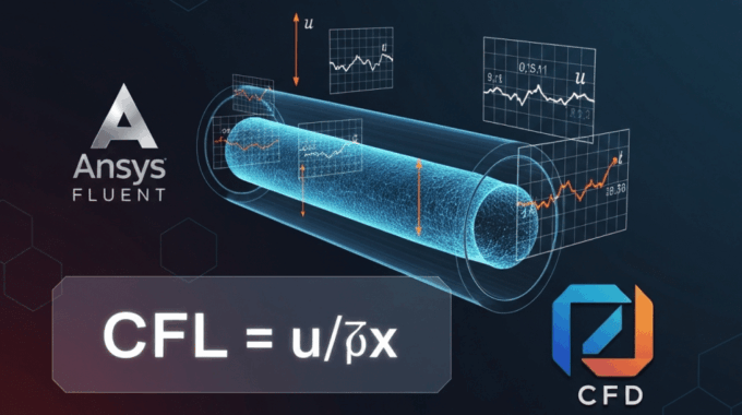
What is the Courant Number? CFL Formula & Calculator Guide

The Courant number, also called the CFL number, measures how far flow information travels through a computational cell during one timestep. If the Courant number is too high, your transient CFD simulation can become unstable, inaccurate, or diverge.

As a Senior CFD Educator with over a decade of experience guiding engineers through Ansys Fluent, I have seen many transient simulations fail for one recurring reason: poor CFL number management. In fact, a large percentage of early-stage simulation divergence troubleshooting cases are caused by using a timestep that is too large for the local mesh size and velocity field.

This guide explains the Courant number formula, the physical meaning of the CFL condition, how to calculate the correct timestep in Ansys Fluent, and how to use a Courant number calculator to prevent transient divergence.

By the end, you will know how to:

• Define what is the Courant number
• Understand what is CFL number in CFD
• Use the correct CFL number formula
• Calculate the optimal timestep for Ansys Fluent
• Avoid residual spikes, floating point exceptions, and transient divergence
• Use adaptive time stepping, truncation error tolerance, and local CFL monitoring
• Decide when reducing the CFL number below 10 helps or hurts accuracy

Small Timesteps Killing Your Productivity?

Enforcing a strict Courant Number (CFL < 1) for transient, multiphase, or LES simulations often means running thousands of tiny timesteps. Don’t let your local workstation tie you up for weeks. Run your Ansys Fluent simulations in hours, not days with MR CFD’s dedicated HPC servers.

Why Engineers Choose MR CFD HPC:
⚡ Up to 10x Faster: Access up to 128+ physical cores per server.
💰 Zero Hardware Cost: Pay-as-you-go or monthly rentals. No $20k workstation needed.
🛠️ CFD Expert Support: Our team helps optimize your Fluent setup for maximum parallel efficiency.

Get ANSYS HPC Pricing  →

What Is the Courant Number?

The Courant number is a dimensionless number that compares the physical distance traveled by flow information in one timestep to the size of a computational cell.

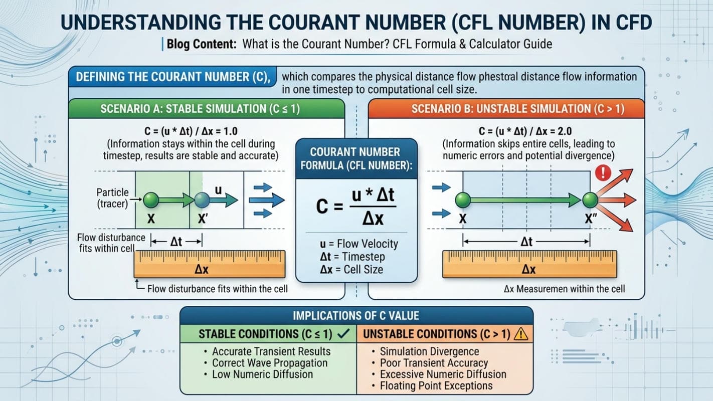
The Courant number tells you whether your timestep is physically reasonable for your mesh and velocity field. It is one of the most important stability parameters in transient CFD.

In simple terms:

The Courant number shows how many cells a fluid particle, wave, or flow disturbance crosses during one timestep.

If the value is too large, the solver may skip over important flow information. This can cause:

• Simulation divergence
• Residual spikes
• Poor transient accuracy
• Excessive numeric diffusion
• Floating point exceptions in Fluent
• Unstable pressure and velocity fields

The Courant number is also known as the CFL number, named after Courant, Friedrichs, and Lewy.

What Is CFL Number in CFD?

Short answer is The CFL number is another name for the Courant number. It controls whether the numerical solution respects the physical speed at which information travels through the mesh.

The CFL number acts like a speed limit for your CFD simulation. Imagine your mesh as a city grid and flow information as a delivery truck moving from one cell to the next.

If the truck moves less than one block per timestep, the solver can track it accurately.

If the truck crosses several blocks in one timestep, the solver loses track of the information path. This can cause the solution to become unstable.

Think of the CFL number as the speed limit for your transient simulation. Exceed it, and your solver may crash.

For explicit solvers, the classical stability requirement is usually:

CFL ≤ 1

For implicit solvers, such as many pressure-based transient setups in Ansys Fluent, the solver may tolerate higher CFL numbers, but that does not mean the result is always time-accurate.

High CFL values can still smear transient events, increase numeric diffusion, and hide important physics.

Courant Number Formula: Derivation and Calculation

The standard Courant number formula is CFL = u × Δt / Δx, where u is velocity, Δt is timestep, and Δx is cell size.

The basic Courant number formula comes from the 1D advection equation:

∂φ/∂t + u ∂φ/∂x = 0

This equation describes how a scalar quantity, such as temperature, velocity, species concentration, or volume fraction, is transported by a velocity field.

When the equation is discretized in time and space, the critical stability term becomes:

u Δt / Δx

This term is the Courant number.

CFL Number Formula

CFL = (u × Δt) / Δx

Where:

• CFL = Courant number or CFL number
• u = local flow velocity
• Δt = timestep size
• Δx = local cell size in the flow direction

For stability in classical explicit time integration:

CFL ≤ 1

This means the information should not travel more than one cell length during a single timestep.

What Is the CFL Number Formula in 3D CFD?

In 3D CFD, the CFL number formula includes all velocity components and cell dimensions in the x, y, and z directions.

For a three-dimensional simulation, the Courant number formula becomes:

CFL = Δt × ( |u|/Δx + |v|/Δy + |w|/Δz )

Where:

• u, v, w are velocity components in the x, y, and z directions
• Δx, Δy, Δz are local cell dimensions
• Δt is the timestep

This is why grid resolution directly controls timestep selection. If you refine your mesh and reduce the smallest cell size, the same timestep produces a larger CFL number.

That is one of the most common mistakes in Ansys Fluent: engineers refine the mesh but forget to reduce the timestep.

Stop Waiting, Start Simulating

Strict CFL limits slowing down your project? Rent dedicated Ansys Fluent HPC servers and cut your simulation time from weeks to hours. Enterprise performance, fixed monthly pricing, no hardware purchase needed.

Get ANSYS HPC Pricing  →

What Is the Courant Number Formula for Incompressible Flow?

For incompressible flow, the Courant number is based mainly on fluid velocity because pressure information is not transported as acoustic waves in the same way as compressible flow.

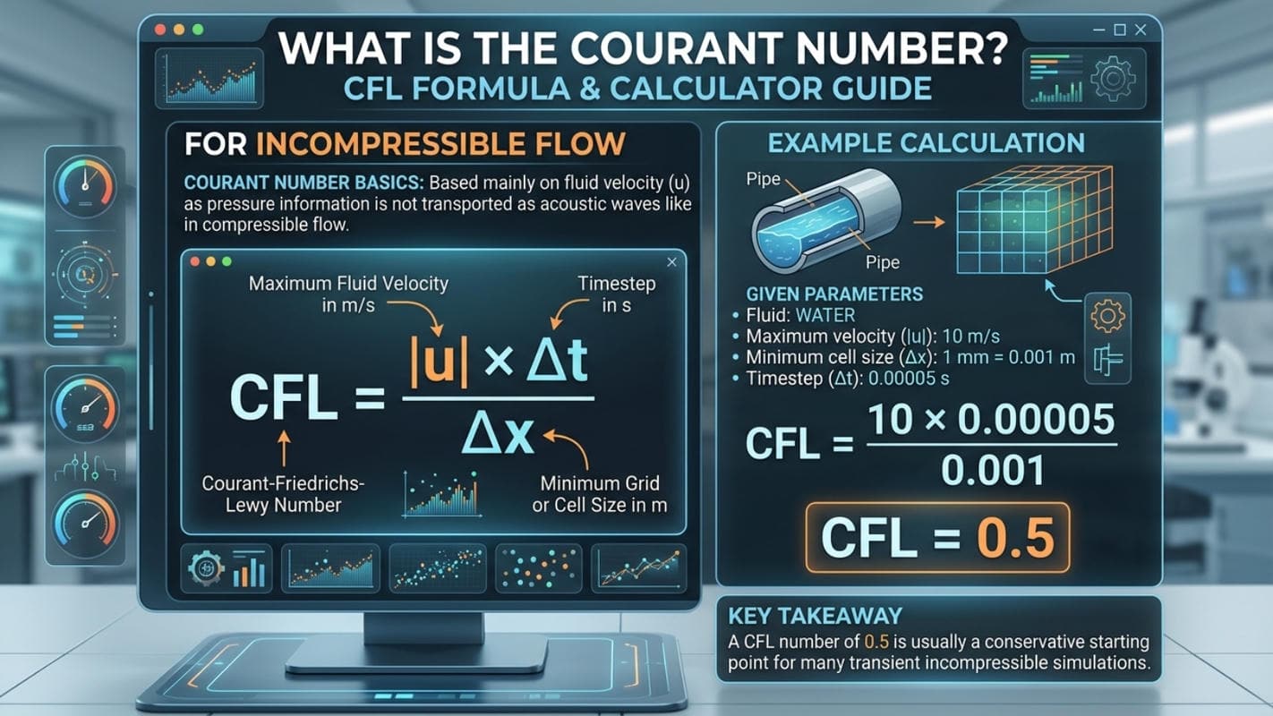
For incompressible flow:

CFL = (|u| × Δt) / Δx

Example:

Water flows through a pipe at:

• Maximum velocity: 10 m/s
• Minimum cell size: 1 mm = 0.001 m
• Timestep: 0.00005 s

CFL = (10 × 0.00005) / 0.001 = 0.5

A CFL number of 0.5 is usually a conservative starting point for many transient incompressible simulations.

What Is the CFL Number Formula for Compressible Flow?

For compressible flow, the CFL number formula must include both fluid velocity and speed of sound because acoustic waves carry information through the domain.

For compressible flow:

CFL = ((|u| + c) × Δt) / Δx

Where:

• u = local flow velocity
• c = local speed of sound
• Δt = timestep
• Δx = local cell size

This is critical for high-speed CFD.

Example:

Air flows over an airfoil at:

• Velocity: 680 m/s
• Speed of sound: 340 m/s
• Cell size: 0.001 m
• Target CFL: 1

The relevant information speed is:

|u| + c = 680 + 340 = 1020 m/s

The timestep should be:

Δt = (1 × 0.001) / 1020 = 9.8e-7 s

Ignoring the speed of sound in compressible simulations is one of the fastest ways to create residual spikes, instability, or floating point exceptions in Fluent.

What CFL Values Should You Use in Ansys Fluent?

In Ansys Fluent, use low CFL numbers for time-accurate transient simulations and higher values only when the solver and physics can tolerate them.

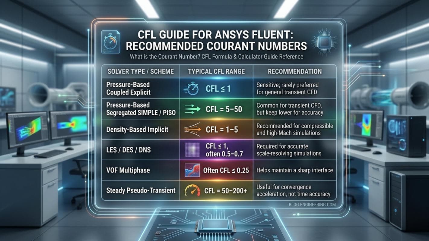
The correct CFL number depends on the solver type, time discretization, turbulence model, mesh quality, and whether the case is steady or transient.

Solver Type / Scheme	Typical CFL Range	Recommendation
Pressure-Based Coupled Explicit	CFL ≤ 1	Sensitive; rarely preferred for general transient CFD
Pressure-Based Segregated SIMPLE / PISO	CFL = 5–50	Common for transient CFD, but keep lower for accuracy
Density-Based Implicit	CFL = 1–5	Recommended for compressible and high-Mach simulations
LES / DES / DNS	CFL ≤ 1, often 0.5–0.7	Required for accurate scale-resolving simulations
VOF Multiphase	Often CFL ≤ 0.25	Helps maintain a sharp interface
Steady Pseudo-Transient	CFL = 50–200+	Useful for convergence acceleration, not time accuracy

Fluent-Specific Warning: “Reducing the CFL Number Below 10 Is Not Recommended Fluent”

In Ansys Fluent, reducing the CFL number below 10 is not universally bad. It depends on whether your goal is stability, accuracy, or steady-state convergence acceleration.

The phrase “reducing the CFL number below 10 is not recommended Fluent” can be misleading. For steady-state pseudo-transient calculations, very low CFL values may slow convergence and increase computational cost. However, for time-accurate transient CFD, LES, VOF, compressible flow, or cases with strong gradients, reducing CFL below 10 is often necessary.

Use this rule:

• For steady pseudo-transient Fluent simulations, CFL below 10 may be inefficient.
• For transient simulations, CFL below 10 is often recommended for accuracy.
• For LES/DES/DNS, use CFL ≤ 1.
• For VOF multiphase flow, use CFL ≤ 0.25 near the interface.

Very small timesteps can increase runtime and accumulated numeric diffusion, but too large a timestep can cause divergence or smear transient physics.

How Do You Set the Timestep in Fluent’s Pressure-Based Transient Solver?

In Fluent’s pressure-based transient solver, you usually set the timestep directly, then verify the resulting CFL number using mesh size and maximum velocity.

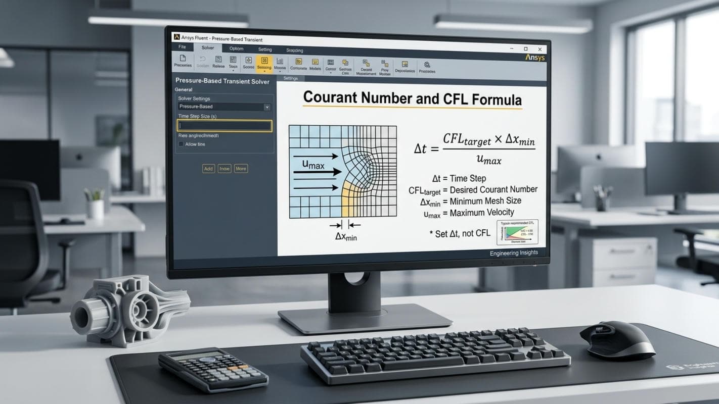
For pressure-based transient simulations in Ansys Fluent, you typically define:

Time Step Size = Δt

You do not usually enter the Courant number directly. Instead, calculate the timestep using:

Δt = (CFLtarget × Δxmin) / umax

Where:

• CFLtarget = desired Courant number
• Δxmin = smallest controlling cell size
• umax = maximum expected velocity

Worked Example

You are simulating water flow in a pipe:

• Maximum velocity: 5 m/s
• Minimum cell size: 0.001 m
• Target CFL: 0.5

Δt = (0.5 × 0.001) / 5 Δt = 0.0001 s

In Ansys Fluent, go to:

Solution > Run Calculation > Time Step Size

Enter:

0.0001

This is the foundation of calculating optimal timestep for preventing transient divergence.

How Do You Enable Adaptive Time Stepping in Fluent?

Enable Adaptive Time Stepping in Fluent through Solution Controls and set minimum timestep, maximum timestep, and truncation error tolerance.

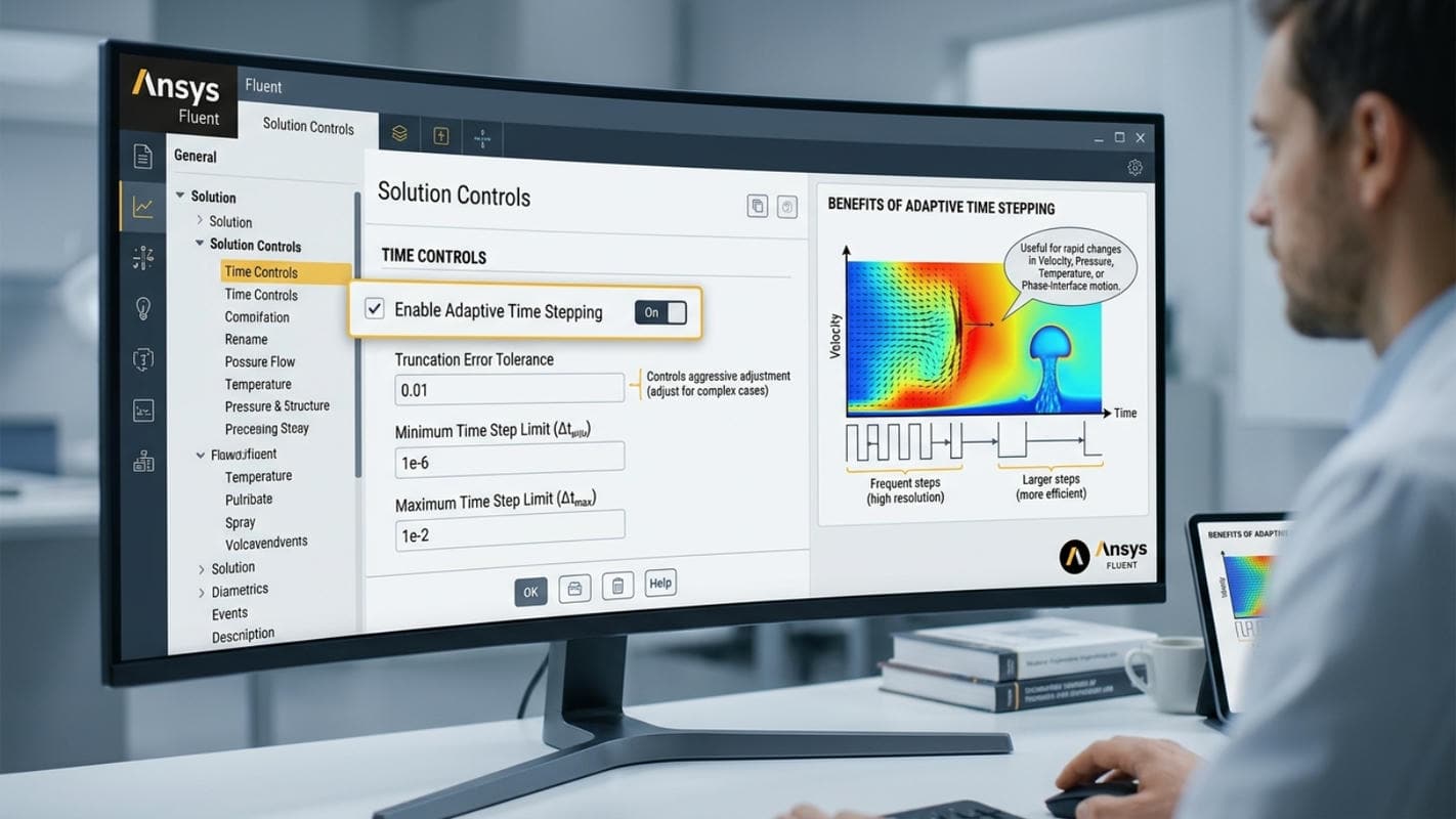
Adaptive time stepping is useful when velocity, pressure, temperature, or phase-interface motion changes rapidly during the simulation.

In Ansys Fluent:

1. Go to Solution > Solution Controls
2. Open the solver/time controls section
3. Enable Adaptive Time Stepping
4. Set Truncation Error Tolerance
5. Define minimum and maximum timestep limits

The truncation error tolerance controls how aggressively Fluent adjusts the timestep. A value around 0.01 is often a reasonable starting point, but complex cases may need tuning.

Benefits of Adaptive Time Stepping

• Improves robustness during high-gradient events
• Reduces timestep automatically near rapid transients
• Saves computational time when the flow becomes quasi-steady
• Helps with stabilizing residuals

Risks of Adaptive Time Stepping

• Can skip important transient events if maximum timestep is too large
• Adds another parameter to monitor
• May not fully prevent local CFL violations in poor mesh regions

I recommend adaptive time stepping especially for:

• Multiphase flow
• Reacting flow
• Valve opening or closing
• Sloshing
• Strong pressure waves
• Moving mesh simulations

Struggling with Transient Divergence?

Let our engineers review your timestep, mesh, and local CFL number distribution. We provide simulation divergence troubleshooting with a 24-hour turnaround time.

CFD Consultation (#4)

Get a free project feasibility study

You'll talk to a senior CFD engineer, not a salesperson.

Full Name

Email (It's better to enter your Work E-mail)

What is your Job role?

Engineer

Manager

Student / Researcher

Other

Submit Request

How Do You Calculate the Optimal Timestep for Your Geometry?

To calculate the optimal timestep, identify the smallest cell size, estimate the maximum velocity, choose a target CFL number, and apply the timestep formula.

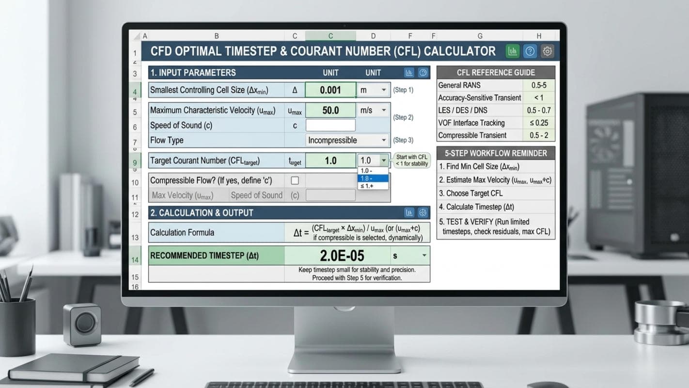
Use this 5-step workflow for calculating optimal timestep in transient CFD.

Step 1: Find the Smallest Controlling Cell Size

In Ansys Fluent, check the mesh information using:

Domain > Mesh Info

or in Fluent Meshing:

Mesh > Info > Size

Find the minimum cell size or the smallest cell length in the main flow direction.

This value is your critical:

Δxmin

Step 2: Estimate the Maximum Characteristic Velocity

For incompressible flow, use:

umax

For compressible flow, use:

umax + c

where c is the local speed of sound.

For moving mesh cases, use relative velocity:

|ufluid – umesh|

Step 3: Choose a Target CFL Number

Recommended starting values:

• General transient RANS: CFL = 0.5–5
• Accuracy-sensitive transient: CFL < 1
• LES/DES/DNS: CFL = 0.5–0.7
• VOF interface tracking: CFL ≤ 0.25
• Compressible transient: CFL = 0.5–2

Step 4: Calculate the Timestep

Use:

Δt = (CFLtarget × Δxmin) / umax

For compressible flow:

Δt = (CFLtarget × Δxmin) / (umax + c)

Step 5: Test and Verify

Run only 10–20 timesteps first.

Monitor:

• Continuity residual
• Momentum residuals
• Energy residual
• Turbulence residuals
• Maximum CFL number
• Flow monitors
• Mass imbalance

If residuals explode, reduce the timestep by 2–5x and inspect local CFL contours. 

What Role Does Mesh Quality Play in CFL Stability?

Poor mesh quality can create local CFL number spikes even when the global CFL appears safe.

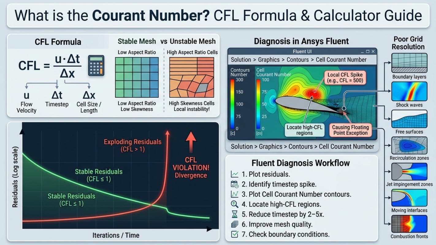Your mesh controls the denominator of the CFL formula. If a few cells are extremely small, skewed, or stretched, they can dominate the timestep stability limit.

High Aspect Ratio Cells

Long and thin cells can cause problems because the CFL condition may be controlled by the smallest cell dimension.

If the aspect ratio is very high, for example greater than 100:1, the timestep required for stability may become impractically small.

High Skewness Cells

Cells with high skewness, especially above 0.85, can produce local instability.

A simulation may show a reasonable global CFL but still diverge because one small skewed region has a local CFL number of 200, 500, or higher.

Poor Grid Resolution

Insufficient grid resolution near high-gradient zones can also cause instability and inaccurate transient behavior.

Important regions include:

• Boundary layers
• Shock waves
• Free surfaces
• Recirculation zones
• Jet impingement zones
• Moving interfaces
• Combustion fronts

Always inspect local Cell Courant Number contours, not just global reports.

How Do You Diagnose CFL-Related Divergence in Fluent?

CFL-related divergence usually appears as sudden residual spikes, unstable flow variables, or floating point exceptions in Fluent after a timestep increase.

Common signs of CFL-related instability include:

• Residuals jumping to 1e+06 or higher
• Continuity residual exploding first
• Velocity magnitude becoming unrealistic
• Temperature or pressure becoming unbounded
• Courant number hotspots in small cells
• Floating point exception in Fluent
• Divergence immediately after flow acceleration

Fluent Diagnosis Workflow

1. Plot residuals.
2. Identify the timestep where residuals spike.
3. Plot Cell Courant Number contours.
4. Locate high-CFL regions.
5. Reduce timestep by 2–5x.
6. Improve mesh quality if local CFL remains extreme.
7. Check boundary conditions and initialization.

In Ansys Fluent, go to:

Solution > Graphics > Contours

Then select:

Cell Courant Number

This shows where your local CFL is too high.

What Is the Difference Between Global and Local CFL Number?

The global CFL number summarizes the domain, while local CFL shows the value inside each individual cell.

A global CFL value can hide dangerous local regions.

For example:

• Reported global CFL: 8
• Local CFL in tiny skewed cells: 450

The solver may diverge because of the local hotspot, even though the reported average seems acceptable.

For this reason, always plot Cell Courant Number contours during simulation divergence troubleshooting.

How Does Turbulence Modeling Affect the CFL Number?

RANS models may tolerate higher CFL numbers, while LES, DES, and DNS require stricter CFL control for stability and accuracy.

RANS Models

Common RANS models include:

• k-epsilon
• k-omega
• SST k-omega
• Reynolds Stress Model

These models often use implicit treatment for source terms, which may improve stability. However, high CFL values can still reduce temporal accuracy.

LES, DES, and DNS

For scale-resolving simulations, the timestep must resolve turbulent structures.

Recommended CFL values:

CFL ≤ 1

Often:

CFL = 0.5–0.7

For high-fidelity LES or DNS, CFL management is not optional. It is part of the physics resolution requirement.

This is a core topic in advanced Ansys Fluent training for transient and scale-resolving simulations.

How Does CFL Affect Numeric Diffusion in CFD?

Very high CFL numbers can smear transient flow features, while extremely small timesteps can increase accumulated numerical error and computational cost.

Numeric diffusion CFD problems appear when sharp gradients become artificially smeared by the numerical method.

High CFL can worsen:

• Shock smearing
• Interface diffusion in VOF
• Vortex decay
• Temperature-front smearing
• Species-gradient smearing
• Loss of transient peak values

However, extremely tiny timesteps are not always ideal either. Every timestep introduces some numerical error. If you take too many unnecessary timesteps, those errors can accumulate.

The goal is not simply the smallest timestep possible.

The goal is:

A timestep small enough for stability and accuracy, but large enough for practical runtime.

How Do You Handle CFL in Moving Mesh and Overset Simulations?

In moving mesh simulations, calculate the CFL number using the relative velocity between fluid and mesh.

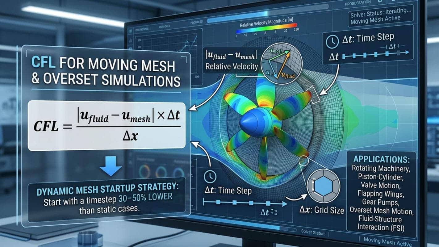
For Fluent dynamic mesh, overset mesh, sliding mesh, and deforming mesh cases, the mesh itself moves. Therefore, the relevant velocity is not simply fluid velocity.

Use:

CFL = (|ufluid – umesh| × Δt) / Δx

This is important in:

• Rotating machinery
• Piston-cylinder simulations
• Valve motion
• Flapping wings
• Gear pumps
• Overset mesh motion
• Fluid-structure interaction

For dynamic mesh cases, start with a timestep 30–50% lower than a comparable static mesh setup.

What CFL Number Should You Use for Multiphase Flow?

Multiphase simulations, especially VOF, require low CFL numbers to preserve interface sharpness and prevent instability.

Recommended values:

Multiphase Model	Suggested CFL
VOF	CFL ≤ 0.25
Eulerian Model	CFL ≤ 1
Mixture Model	CFL ≤ 5

For VOF simulations, the interface can become smeared if the timestep is too large. A low CFL helps reduce interface diffusion and improves phase-front resolution.

This is especially important in:

• Sloshing
• Wave breaking
• Free-surface flow
• Tank filling
• Oil-water separation
• Spray-interface tracking

What CFL Number Should You Use for Combustion and Reacting Flows?

For reacting flows, the timestep must satisfy both fluid-dynamic CFL limits and chemical timescale requirements.

Combustion simulations are difficult because the flow and chemistry may have very different timescales.

You must resolve:

• Convective transport
• Acoustic waves, if compressible
• Heat release
• Species transport
• Chemical kinetics
• Flame propagation

Even if the Courant number is acceptable, the timestep may still be too large for reaction kinetics.

In reacting-flow CFD, monitor:

• Temperature residuals
• Species residuals
• Heat release rate
• Flame speed
• Maximum temperature
• Local CFL

What CFL Number Should You Use for Supersonic and Hypersonic Flow?

Supersonic and hypersonic simulations usually require density-based solvers, coupled energy-flow solution, and low initial CFL numbers.

Best practices:

1. Use the Density-Based Solver
2. Include speed of sound in the CFL number formula
3. Start with CFL = 0.5–2
4. Use local time stepping for steady initialization
5. Solve flow and energy equations in a coupled manner
6. Refine the mesh near shocks and boundary layers

For steady hypersonic cases, local time stepping can accelerate convergence. For transient hypersonic cases, use physical timesteps based on the compressible CFL formula.

How Do You Use UDFs to Enforce Local CFL Limits?

A Fluent UDF can monitor local CFL numbers and dynamically adjust the timestep to keep the simulation stable.

For advanced control, you can write a User-Defined Function that checks each cell, finds the maximum local CFL, and adjusts the timestep.

Conceptual example:

C Language:

/* Sample UDF to control timestep based on max CFL */ #include "udf.h" DEFINE_ADJUST(adjust_timestep, domain) { real max_cfl = 0.0; real target_cfl = 0.8; /* Loop over all cell threads and cells */ /* Compute local cell_cfl */ /* Update max_cfl if cell_cfl > max_cfl */ if (max_cfl > 0.0) { real current_dt = CURRENT_TIMESTEP; /* Adjust next timestep */ Set_Time_Step(target_cfl / max_cfl * current_dt); } }

This strategy is useful for:

• LES
• VOF
• Moving mesh
• Reacting flow
• Rapid valve motion
• Shock-dominated compressible flow

A custom UDF provides more control than built-in adaptive time stepping, but it requires careful testing and validation.

Common Mistakes Engineers Make with the Courant Number

The most common CFL mistakes are using the global CFL only, ignoring speed of sound, trusting implicit solvers too much, and forgetting to update timestep after mesh refinement.

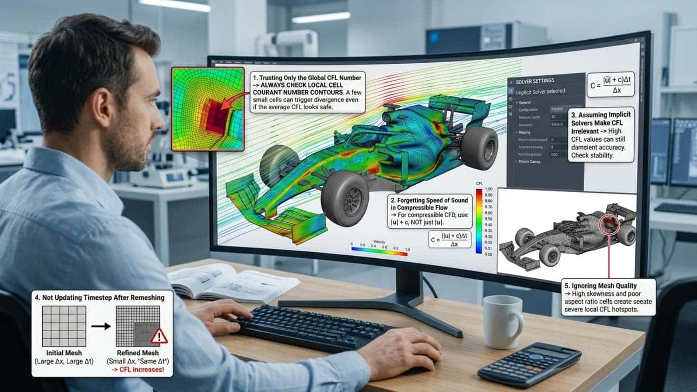
Avoid these mistakes:

1. Trusting Only the Global CFL Number

Always check local Cell Courant Number contours.

A few small cells can trigger divergence even if the average CFL looks safe.

2. Forgetting Speed of Sound in Compressible Flow

For compressible CFD, use:

|u| + c

not just:

|u|

3. Assuming Implicit Solvers Make CFL Irrelevant

Explicit vs implicit solvers differ in stability behavior, but implicit solvers are not magic.

High CFL values can still damage transient accuracy.

4. Not Updating Timestep After Remeshing

If the mesh is refined, Δx decreases.

If timestep remains unchanged, the CFL number increases.

5. Ignoring Mesh Quality

High skewness and poor aspect ratio cells can create severe local CFL hotspots.

How Can MR CFD Help with CFL and Transient Simulation Stability?

 helps engineers diagnose CFL number problems, optimize timestep settings, improve mesh quality, and stabilize transient Ansys Fluent simulations.

Our services include:

• Simulation divergence troubleshooting
• Fluent case-file review
• Mesh and timestep optimization
• CFD consulting services
• Custom Ansys Fluent training
• Advanced transient CFD workshops
• UDF development for adaptive timestep control
• ANSYS HPC support for transient simulations

A recent automotive client had a transient underhood thermal simulation that diverged repeatedly. After reviewing the case, we identified local CFL number violations caused by poor mesh quality in a narrow region. By improving the mesh and adjusting timestep controls, the simulation became stable and runtime was reduced significantly.

Master Transient Simulations

Go beyond the basics. Enroll in our Transient CFD Mastery course to learn advanced timestep control, UDF-based CFL management, LES setup, and scale-resolving simulation workflows.

View Course Curriculum

Frequently Asked Questions About Courant Number and CFL Number

What happens if my CFL number exceeds 1 in an implicit solver?

An implicit solver may not diverge immediately when CFL > 1, but temporal accuracy can decrease.

Implicit solvers are more stable than explicit solvers, but a high CFL number can smear transient features and miss short-lived physical events.

For time-accurate transient simulations, keep CFL reasonably low. For many Fluent cases, CFL < 10 is a good practical upper target, while LES and VOF require much lower values.

Can I use a constant timestep for all transient simulations?

No. A constant timestep is useful for periodic or stable flows, but adaptive time stepping is better for flows with rapidly changing timescales.

Use a constant timestep for:

• Vortex shedding
• Periodic flows
• Fully developed transient cycles
• Controlled benchmark studies

Use adaptive time stepping for:

• Valve motion
• Multiphase flow
• Reacting flow
• Shock propagation
• Startup and shutdown processes

How do I choose between first-order and second-order time discretization?

Use Second Order Implicit for accuracy, but consider First Order Implicit for the first few timesteps of difficult simulations.

First-order time discretization is more robust but more diffusive.

Second-order time discretization is more accurate and should be used for final transient results.

A practical workflow is:

1. Start with First Order Implicit for 5–20 timesteps
2. Stabilize residuals
3. Switch to Second Order Implicit
4. Continue with validated timestep size

What is the difference between Courant number and CFL number?

There is no practical difference. The CFL number is the same stability parameter as the Courant number.

The term CFL comes from Courant, Friedrichs, and Lewy. In CFD software and literature, both terms are often used interchangeably.

What is the best CFL number for LES and DNS?

For LES and DNS, use CFL ≤ 1, and often target CFL = 0.5–0.7.

LES and DNS resolve unsteady turbulent structures directly, so the timestep must be small enough to capture eddy motion accurately.

High CFL values can destroy the quality of scale-resolving simulations.

What is the CFL limit for VOF in Ansys Fluent?

For VOF simulations in Ansys Fluent, use CFL ≤ 0.25 near the interface for sharp and stable phase tracking.

VOF is sensitive to timestep size because the interface position must be transported accurately. A high CFL can smear the interface or cause instability.

How do I calculate CFL for non-Newtonian fluids?

The CFL formula is the same for non-Newtonian fluids, but estimating maximum velocity can be more difficult.

Use:

CFL = (|u| × Δt) / Δx

The challenge is that shear-thinning or shear-thickening behavior can create unexpected local velocity peaks.

Always monitor local velocity and local Cell Courant Number after initialization.

Can MR CFD review my Fluent setup to optimize CFL settings?

Yes. MR CFD can review your Ansys Fluent case file and recommend timestep, mesh, solver, and CFL settings.

Our engineering team can help with:

• Fixing floating point exceptions in Fluent
• Preventing transient divergence
• Improving mesh quality
• Selecting timestep size
• Optimizing solver controls
• Stabilizing residuals

Final Takeaway

Short answer is The Courant number is one of the most important controls for stable and accurate transient CFD. If you understand the CFL formula, monitor local CFL values, and calculate timestep correctly, you can prevent many Fluent divergence problems.

The key equation is:

CFL = (u × Δt) / Δx

For compressible flow:

CFL = ((u + c) × Δt) / Δx

For moving mesh:

CFL = (|ufluid – umesh| × Δt) / Δx

Use low CFL values for accuracy-sensitive transient simulations, LES, VOF, and compressible flow. Use higher CFL values only when appropriate for implicit or steady pseudo-transient calculations.