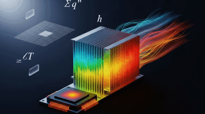
Conjugate Heat Transfer Simulation: Complete CHT Guide

Conjugate Heat Transfer (CHT) simulation is a CFD method that solves fluid flow and solid heat conduction simultaneously, coupling temperature and heat flux at their shared interface. It eliminates assumed heat transfer coefficients, providing true thermal predictions for electronics cooling, turbine blades, and battery thermal management in Ansys Fluent.

A 10°C miscalculation in junction temperature can cost millions in recalled electronics, degraded battery lifespans, or catastrophic turbine blade failure. Yet, countless engineering teams are still forced to guess their Heat Transfer Coefficients (HTC) using decoupled, assumption-heavy thermal models. Stop guessing. This definitive guide distills hard-won insights from over 500+ MR CFD projects into the exact Ansys Fluent CHT workflow used to eliminate thermal guesswork, predict true hotspots, and optimize multiphysics designs.

What Is Conjugate Heat Transfer and Why Does It Matter in Engineering?

At its core, Conjugate Heat Transfer (CHT) is a multiphysics simulation that simultaneously solves heat transfer in both a fluid and a solid domain. The defining feature of a CHT simulation in Ansys Fluent is the fluid-solid thermal coupling: temperature and heat flux are automatically and continuously exchanged at the interface between the fluid and solid parts.

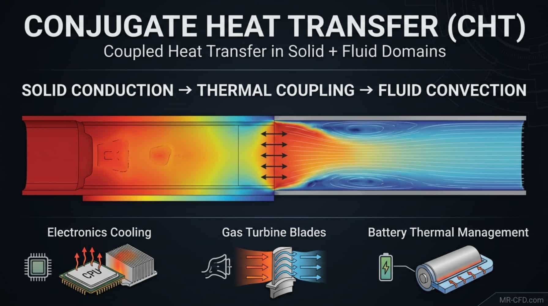
Why can’t you just simulate the fluid or the solid separately? In traditional, decoupled analyses, engineers are forced to make dangerous assumptions. You might assume a constant wall temperature in CFD, or guess an average HTC for a solid thermal FEA model. These “educated guesses” completely miss local flow separations and recirculation zones, leading to massive errors in hotspot prediction. CHT calculates the fluid flow and heat transfer on both sides of the interface dynamically, providing the true temperature distribution without simplified assumptions.

This two-way interaction—where the solid’s temperature affects fluid properties (density, viscosity) and the fluid’s flow dictates solid heat removal—is non-negotiable in high-performance applications:

• High-Power Electronics Cooling: The junction temperature of a modern CPU depends on heat conducting through the silicon die, the thermal interface material (TIM), and the heatsink base before being carried away by air.
• Gas Turbine Blades: Metal temperatures dictating blade lifespan are the direct result of hot external gases and cool internal serpentine passages interacting through the blade wall.
• Battery Thermal Management: EV battery safety relies on maintaining uniform cell temperatures. CHT simulates how heat generated within solid cells transfers to liquid coolant plates, preventing thermal runaway.

Is CHT the Same as CFD? Understanding CHT CFD Coupling

A common point of confusion is the relationship between standard CFD and CHT. CHT is a specialized type of CFD simulation. Standard CFD solves the Navier-Stokes equations for fluid flow and typically applies a fixed thermal boundary condition (like a static temperature or a user-defined HTC) at the walls.

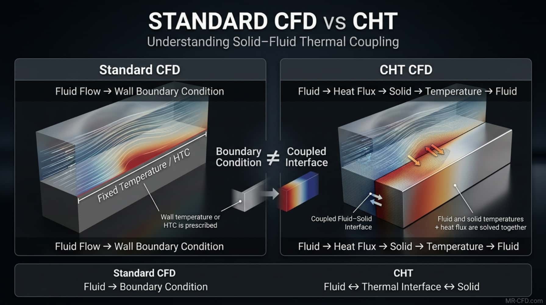
CHT extends standard CFD by adding solid conduction physics to the solver. Instead of applying a boundary condition at the wall, the wall becomes a coupled interface. The CFD solver calculates the fluid-side heat flux, passes it to the solid domain to solve Fourier’s law of conduction, and iterates until thermal equilibrium is reached. If you are searching for “CHT CFD” methodologies, you are looking for this exact coupled solver approach.

Conjugate Heat Transfer Analysis vs. Decoupled FEA/CFD

Understanding when to invest computational resources into a full conjugate heat transfer analysis versus a simpler method is a critical engineering skill. The key difference lies in interface treatment.

Feature	Conjugate Heat Transfer (CHT)	Decoupled Thermal Analysis (CFD or FEA)
Interface Treatment	Domains coupled; temperature/flux solved dynamically.	User specifies fixed BCs (e.g., assumed HTC).
Accuracy	High; captures true physical interaction & local hotspots.	Lower; entirely dependent on user assumptions.
Computational Cost	Higher; solves energy equations in both domains.	Lower; solves only one domain.
Applicability	Essential when solid conduction limits design or HTC is unknown.	Early-stage design or negligible solid thermal resistance.

The Cost of Poor Thermal Assumptions

Engineers must justify the computational expense of CHT to management. Relying on decoupled assumptions carries a hidden “cost of poor CHT” that impacts the bottom line.

Engineering Impact	Decoupled Assumption (Guessing HTC)	CHT Reality (Coupled Simulation)
Material Costs	Over-engineering heatsinks by 20-30% due to safety factors.	Optimized material usage via exact thermal resistance mapping.
Prototyping	3-4 physical thermal iterations to find hidden hotspots.	1 physical prototype for final validation only.
Product Lifespan	Missed localized hotspots lead to premature field failures.	Accurate junction temperature prediction ensures warranty compliance.
Cost of Failure	$500k+ in recalled batches or turbine blade replacements.	$0 (Caught in the virtual design phase).

Still Guessing at Heat Transfer Coefficients?

See how 500+ CHT projects replaced assumption-based thermal analysis with real coupled results.

CFD Consultation (#4)

Get a free project feasibility study

You'll talk to a senior CFD engineer, not a salesperson.

Full Name

Email (It's better to enter your Work E-mail)

What is your Job role?

Engineer

Manager

Student / Researcher

Other

Submit Request

What Are the Fundamental Physics Governing Conjugate Heat Transfer?

A CHT simulation doesn’t invent new physics; it unifies the governing equations for fluid flow and heat conduction into a single, coupled solver.

How Do Fluid Domain Energy Equations Work in CHT Simulations?

In the fluid, heat moves through two primary mechanisms:

1. Convection: Heat carried by bulk fluid motion (dominant in forced-air/liquid cooling).
2. Conduction (Diffusion): Heat transfer through molecular vibrations (critical in slow-moving boundary layers right at the wall).

The steady-state fluid energy equation balances these:

∇ ⋅ (ρ * v * h) = ∇ ⋅ (k_fluid * ∇T) + S_h

(Where the left side is convection, the first right term is diffusion, and S_h represents viscous dissipation).

For turbulent flows, models like SST k-ω or k-ε with enhanced wall treatment are crucial. They accurately predict the turbulent thermal transport and resolve the steep gradients in the viscous sublayer. The fluid’s Prandtl number (Pr) dictates the ratio of momentum diffusivity to thermal diffusivity (Air ≈ 0.7, Water ≈ 7.0).

How Do Solid Domain Heat Conduction Equations Work in CHT Analysis?

Inside the solid, heat transfer is governed purely by conduction (Fourier’s Law):

∇ ⋅ (k_solid * ∇T) = S_v

(Where S_v is volumetric heat generation, e.g., W/m³ in a microchip).

Thermal Conductivity (k_solid) is the driving factor. While metals are isotropic, composites and PCBs are anisotropic (different in-plane vs. through-plane conductivity). Failing to model anisotropic conductivity in PCBs is a leading cause of inaccurate heat spreading predictions. In transient conjugate heat transfer Ansys workflows, the solid’s thermal mass (density × specific heat) becomes vital, governing the time-dependent heat-up and cool-down phases.

What Happens at the Fluid-Solid Interface in CHT Simulations?

The “conjugate” magic happens at the shared boundary, enforced by two conditions:

1. Temperature Continuity: T_fluid_wall = T_solid_wall
2. Heat Flux Continuity: q_solid_wall = q_fluid_wall (or -k_solid * (∂T/∂n)_solid = -k_fluid * (∂T/∂n)_fluid)

Ansys Fluent solves this iteratively. It solves the fluid equations, passes the heat flux to the solid, solves the solid, passes the wall temperature back, and repeats until the interface values converge. This robust methodology ensures physical accuracy.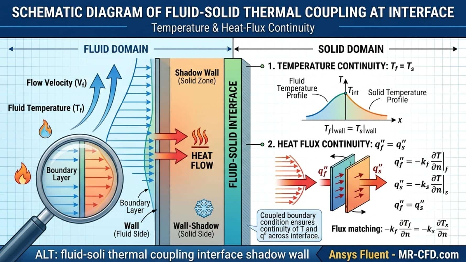

What Are the Most Common Applications of Conjugate Heat Transfer Simulation?

Solid-fluid heat exchange simulation is critical across modern product development.

Electronics Cooling CFD Simulation

With microchip power densities skyrocketing, electronics cooling simulation requires CHT to model the entire thermal pathway from the silicon junction to ambient air.

• Chip Packages: Predicting junction temperature (T_j) through the die, spreader, and substrate.
• Heatsinks: Optimizing fin geometry for maximum dissipation.
• PCBs: Modeling anisotropic heat spreading through copper traces and FR-4.
• TIMs: Capturing the critical temperature drop across thermal interface materials.
• Case in point: Ensuring a 120W CPU stays below a 95°C junction temperature requires testing fin designs and fan curves virtually—something decoupled FEA simply cannot do accurately.

Gas Turbine Blade Cooling

Turbine blades operate above the melting point of their alloys, surviving via sophisticated cooling schemes validated using CHT.

• Internal Passages: Cool air forced through serpentine channels.
• Film Cooling: Cool air injected through micro-holes to insulate the exterior.

Thermal Barrier Coatings (TBCs): Analyzing the extreme temperature drop across ceramic coatings.

• The resulting thermal gradients drive immense thermal stresses. Accurate CHT temperature fields are mandatory inputs for subsequent FEA fatigue analysis.

Heat Exchanger Design

While Effectiveness-NTU methods work for initial sizing, conjugate heat transfer CFD reveals local performance bottlenecks. It accurately calculates thermal resistance through tube walls/fins, investigates fouling layers, and resolves complex flow maldistribution in plate-fin or shell-and-tube geometries that simpler 1D models miss.

Battery Thermal Management CFD

Lithium-ion batteries generate massive heat; excessive temperatures cause degradation or thermal runaway. CHT simulates the exact effectiveness of liquid cold plates, ensures cell-to-cell temperature uniformity (critical for lifespan), and models thermal runaway propagation paths to meet strict EV safety standards.

Electronics, Turbines, or Batteries — Is CHT Right for Your Design?

Talk to an MR CFD specialist about your specific geometry, heat loads, and multiphysics requirements.

CFD Consultation (#4)

Get a free project feasibility study

You'll talk to a senior CFD engineer, not a salesperson.

Full Name

Email (It's better to enter your Work E-mail)

What is your Job role?

Engineer

Manager

Student / Researcher

Other

Submit Request

How Do You Set Up a Conjugate Heat Transfer Simulation in Ansys Fluent?

Getting the details right at each stage is key to achieving an accurate, converged solution. This is the certified workflow we teach in our Ansys Fluent courses.

Geometry Considerations

• Inclusion: Model the fluid domain and all solid parts forming the primary heat conduction path (chip, base, fins).
• Simplification: Remove cosmetic fillets. Be cautious omitting small structural parts; if in doubt, include them.
• Interface Layers: Thin layers like TIMs or TBCs must be modeled as distinct solid bodies or shell conduction zones.
• Fluid Domain: Extract the fluid volume. Extend boundaries upstream (5-10 characteristic lengths) and downstream (10-20 lengths) to allow flow development and prevent reverse flow convergence issues.

Meshing for Conjugate Heat Transfer Analysis

Meshing is the most critical step. A poor mesh guarantees poor thermal results.

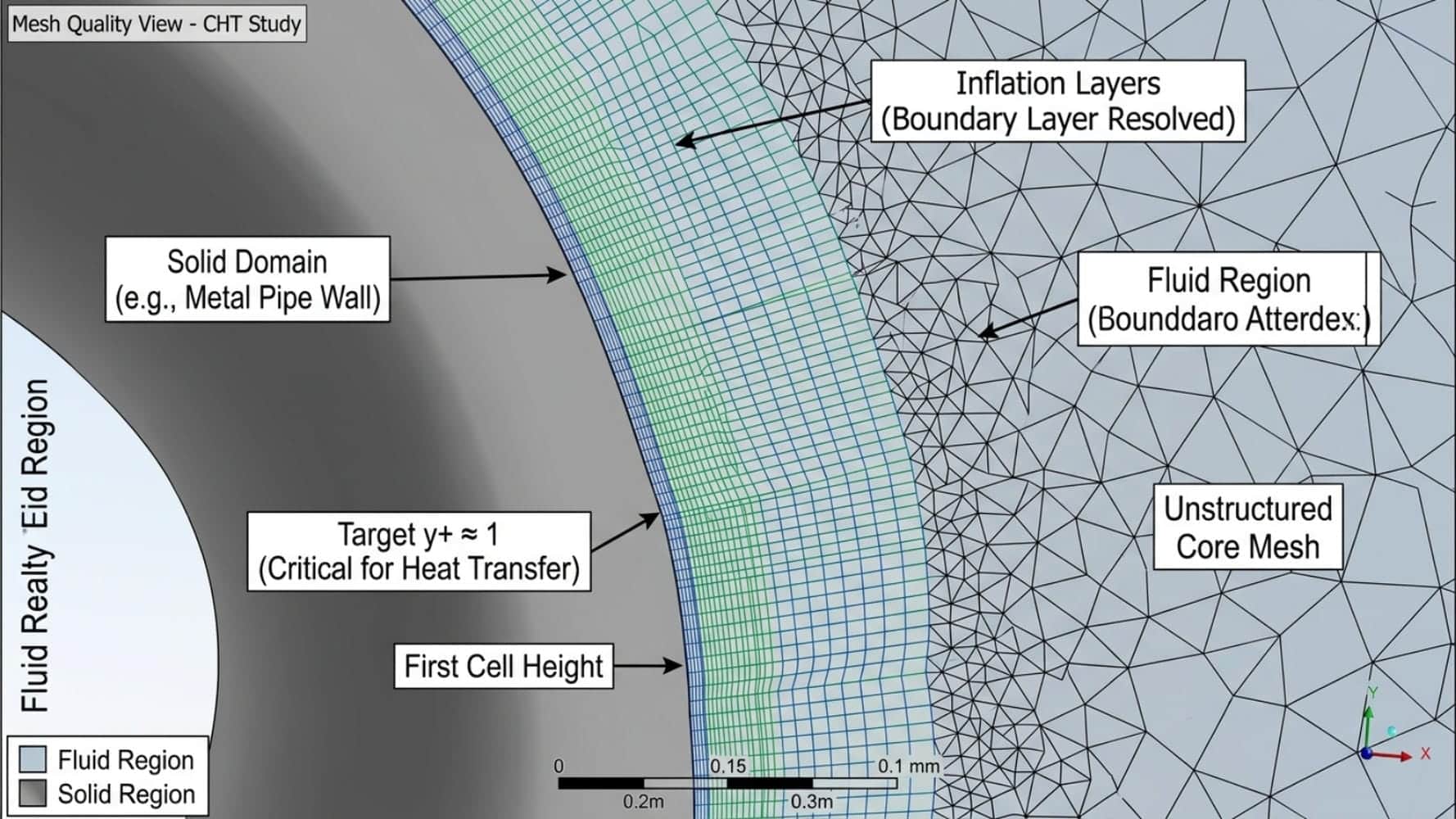
• Interface Conformality: Use a conformal mesh where nodes on the fluid side perfectly match the solid side. Ansys Workbench Meshing handles this automatically via shared topology.
• Boundary Layers (Inflation): You MUST use inflation layers to capture steep thermal gradients. Target a y+ value of ~1 (essential for SST k-ω). Use a minimum of 10-15 inflation layers.
• Solid Mesh: Refine the solid mesh near heat sources or high-flux zones using body sizing controls.
• Quality Metrics: Keep skewness below 0.85 and orthogonal quality above 0.15. Poor elements at the coupled interface are the #1 cause of CHT divergence.

Boundary Conditions

• Fluid: Standard Velocity Inlet / Pressure Outlet.
• Thermal: External walls get fixed Temperature, Heat Flux, or Convection/Radiation conditions.
• Heat Sources: Define volumetric heat generation (W/m³) within the solid cell zone.
• The Interface: Do NOT specify a thermal condition. Fluent automatically recognizes the shared topology as a coupled interface (creating a “shadow wall”) and solves the heat transfer across it.

Material Properties

“Garbage in, garbage out.”

• Fluids: Density, Viscosity, Thermal Conductivity, Specific Heat.
• Solids: Density, Thermal Conductivity, Specific Heat.
• Crucial Note: If temperatures vary by >50°C, use temperature-dependent properties. Constant properties will introduce significant errors in buoyancy-driven natural convection or high-heat-flux scenarios. Don’t forget to model thermal contact resistance at bolted or pressed joints.

Solver Settings & Convergence

• Coupling: The Coupled pressure-velocity scheme is highly robust for CHT.
• Discretization: Minimum Second Order for all equations.
• URFs: CHT can be “stiff” due to differing fluid/solid time scales. If residuals oscillate, drop the Energy URF from 1.0 to 0.8.
• Initialization: Use Hybrid Initialization.
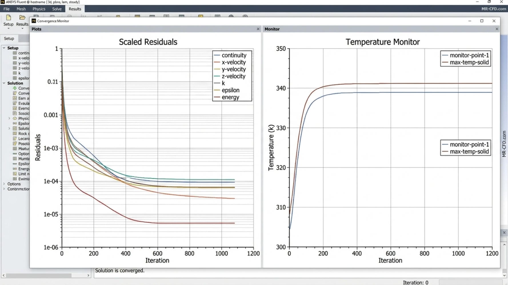
• Monitoring: Never rely solely on residuals. Create monitor points for max heat source temperature and outlet heat flux. The solution is only converged when physical monitors stabilize, even if residuals look flat.

What Is the Complete Workflow for a Heatsink CHT Simulation Example?

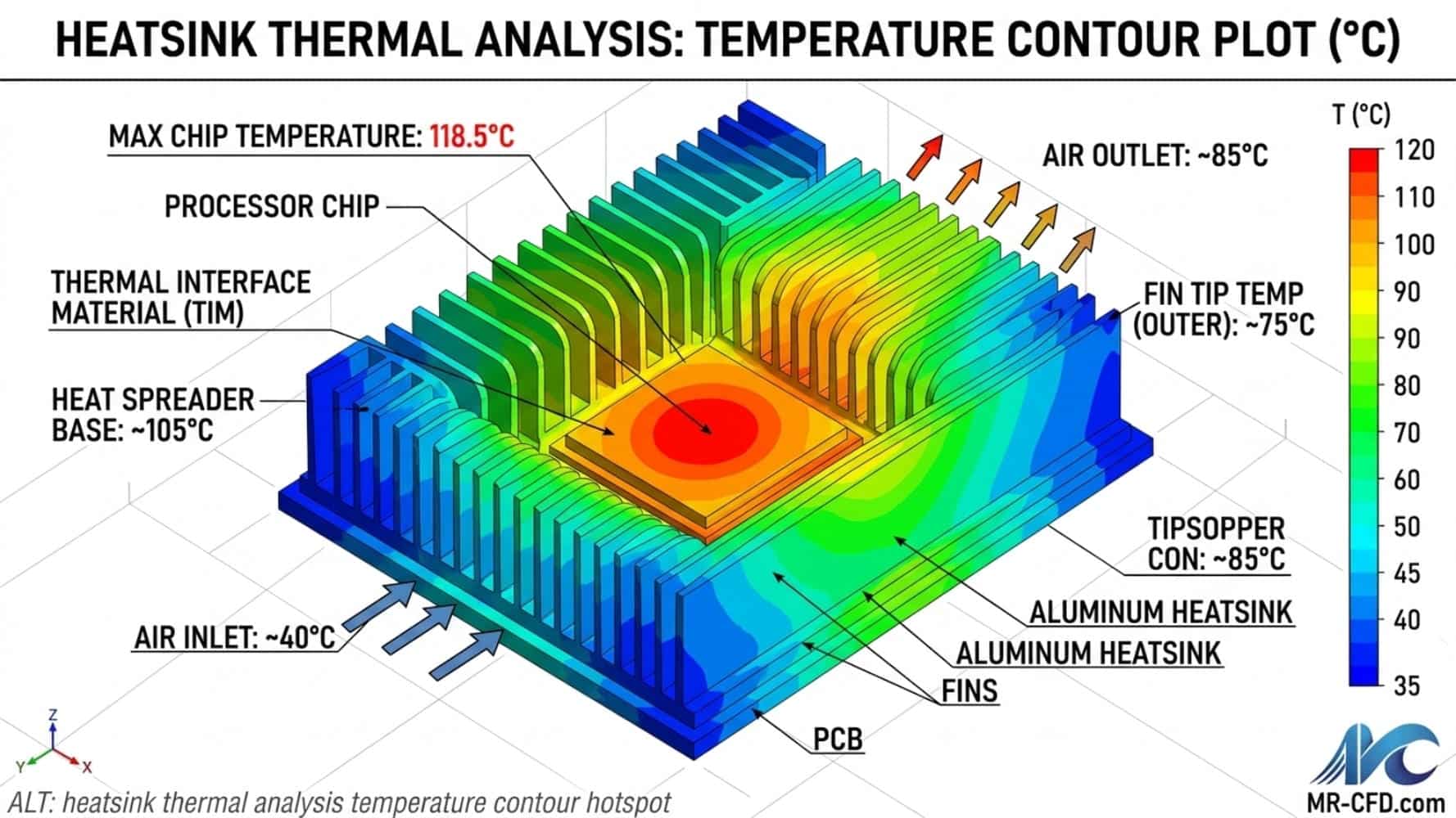
Let’s walk through a practical thermal simulation case study: analyzing an aluminum heatsink cooling a silicon chip.

Problem Definition

• Scenario: 20x20mm silicon chip mounted to an aluminum heatsink. Chip dissipates 50W. Airflow at 2 m/s, ambient 25°C.
• Objectives: Predict max junction temperature, calculate overall thermal resistance (R_th), visualize flow.
• Success Criterion: Max chip temp < 85°C.

Geometry & Mesh Strategy

• Domain: Chip, heatsink, surrounding air. Symmetry plane used to halve compute cost.
• Mesh: Conformal across all interfaces. 15 inflation layers (y+ ≈ 1). Body of influence applied around the heatsink wake. Element count: ~3 million.

Materials & Boundary Conditions

• Inlet: Velocity inlet, 2 m/s, 298.15 K.
• Outlet: Pressure outlet, 0 gauge.
• Heat Source: Volumetric source on silicon chip: 50 W / (0.02 * 0.02 * 0.001 m³) = 1.25e8 W/m³.
• Interfaces: Left as coupled walls (no thermal BC specified).

Solution & Post-Processing

Run with SST k-ω until residuals are flat (Energy < 1e-6) AND chip temp is stable within 0.1°C over 200 iterations.

• Result: Max chip temp = 75°C (Passes <85°C limit).
• Thermal Resistance: R_th = (75 – 25) / 50 = 1.0 °C/W.
• Validation Check: Global heat balance. Net heat rate across boundaries must be <1% of the 50W source term.

Struggling with Mesh Convergence or High Skewness?

Our senior engineers can audit your fluid-solid interface mesh and solver settings in 48 hours.

CFD Consultation (#4)

Get a free project feasibility study

You'll talk to a senior CFD engineer, not a salesperson.

Full Name

Email (It's better to enter your Work E-mail)

What is your Job role?

Engineer

Manager

Student / Researcher

Other

Submit Request

What Are the Most Common Challenges in Conjugate Heat Transfer Simulations?

Why Won’t My CHT Simulation Converge?

1. Poor Mesh Quality: High skewness (>0.9) near the coupled interface causes divergence. Fix: Improve mesh quality reports.
2. Inappropriate Solver Settings: First-order schemes help start the run, but you need Second-Order for accuracy. Fix: Run 50 iterations first-order, then switch. Reduce Energy URF.
3. Physical Instabilities: Natural vortex shedding makes steady-state impossible. Fix: Switch to a pseudo-transient or full transient solver.

Handling Large Temperature Gradients

Steep gradients inside TBCs or the viscous sublayer require extreme resolution. A coarse mesh causes numerical diffusion, “smearing” the peak temperatures. Fix: Use local mesh refinement (Body Sizing) and Adaptive Meshing based on temperature gradients.

Heat Balance Errors

Check Reports -> Fluxes -> Net Heat Transfer Rate. If it’s >1-2% of your total heat input, energy is not conserved.

• Cause 1: Insufficient convergence (run more iterations).
• Cause 2: Incorrect BCs (e.g., accidental adiabatic walls).
• Cause 3: Radiation view factor errors (if using S2S).

Modeling Thermal Contact Resistance

Microscopic air gaps at pressed joints add massive resistance. Ignoring this under-predicts component temperatures. Fix: Model the interface as a Wall with a specified Thermal Resistance (m²K/W) using “Coupled Wall with Shell Conduction” or a thin solid TIM body.

How Do You Validate and Verify Conjugate Heat Transfer Simulation Results?

A colorful plot means nothing if it’s numerically flawed. Verification and Validation (V&V) are mandatory.

Verification (Numerical Accuracy)

The Mesh Independence Study:

1. Run on initial mesh; record max temperature.
2. Refine mesh significantly (reduce element size by 1.5x).
3. Re-run. If the key value changes by <1-2%, the mesh is sufficient. For transient CHT, you must also perform a time-step independence study.

Validation (Physical Reality)

Compare simulation results against experimental data (thermocouples, IR thermography, heat flux sensors). Account for uncertainties in both the physical test and the simulation material properties. For standard geometries, validate against ASME or ERCOFTAC benchmark cases before tackling proprietary designs.

[IMAGE #5 — DESCRIPTION: Before/after comparison showing a decoupled HTC assumption missing a critical hotspot, versus the CHT result accurately capturing it. | TYPE: Comparison Visual | ALT: “decoupled vs CHT simulation hotspot comparison”]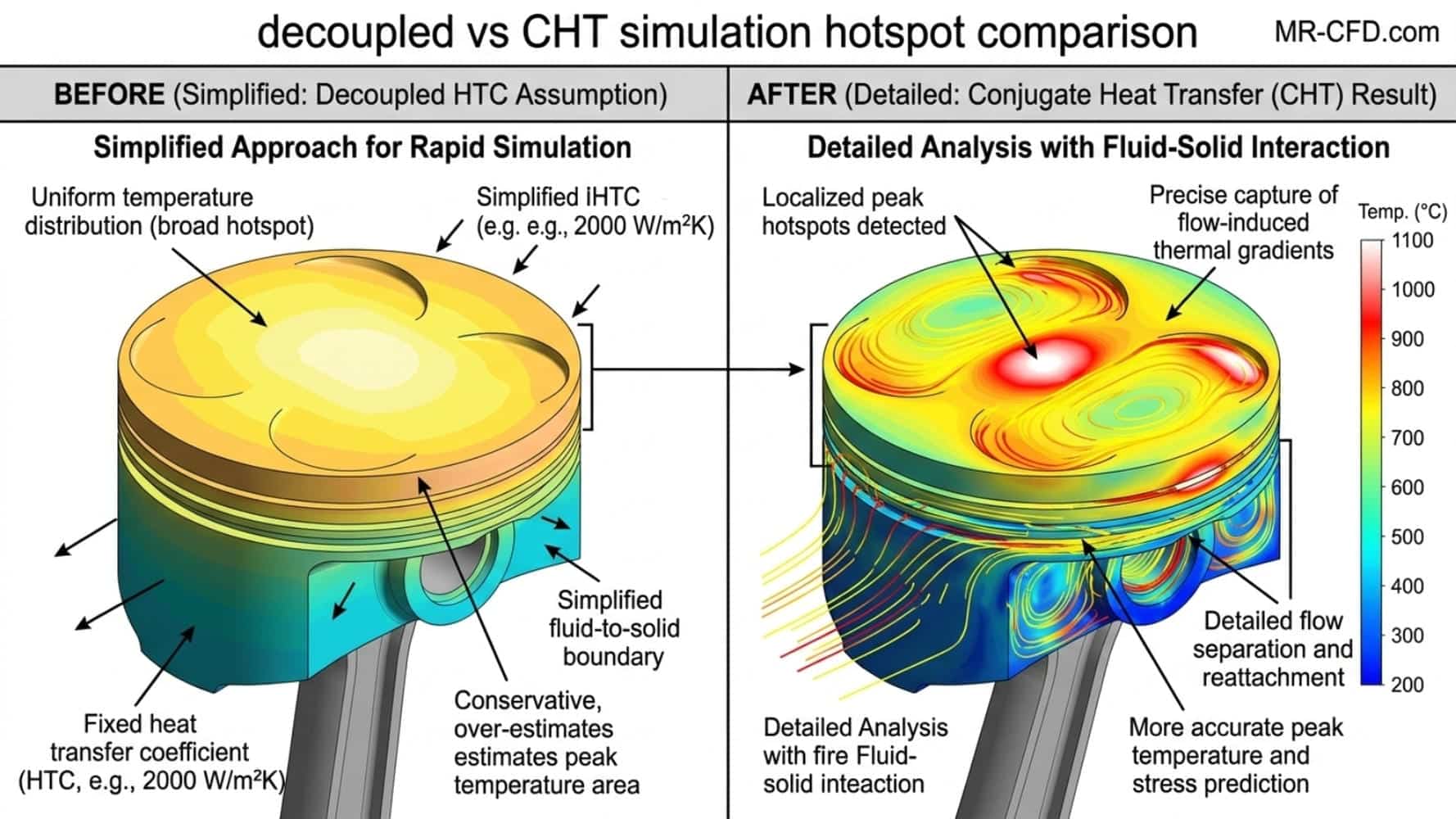

What Advanced Techniques Enhance Conjugate Heat Transfer Simulations?

CHT Model Types in Ansys Fluent

Selecting the right physical model is critical for balancing accuracy and compute cost.

CHT Model Type	When to Use	Key Setting / Consideration	Compute Cost
Steady-State CHT	Continuous operation, nominal thermal loads.	Coupled solver, monitor physical points.	Low to Medium
Transient CHT	Thermal cycling, pulsed power, startup/shutdown.	Solid thermal mass (Cp) dictates time-step size.	High
Radiation-Coupled	High temps (>300°C), vacuum, or natural convection.	S2S (enclosures) or DO (participating media).	High
Moving Parts (FSI)	Rotors, pistons, dynamic thermal contact.	Dynamic mesh (sliding/remeshing) + CHT.	Very High

Including Radiation

Radiation is mandatory in vacuums, sealed enclosures, or high-temp aerospace applications.

• Surface-to-Surface (S2S): Best for non-participating media (air). Expensive upfront for view factors, fast per iteration.
• Discrete Ordinates (DO): Handles participating media (flue gas, glass). Computationally heavy per iteration.

Moving Parts & Deforming Geometry

Combining CHT with dynamic meshing (sliding mesh for motors, layering for pistons) allows for thermal analysis of moving assemblies. These are highly complex multiphysics simulations typically reserved for advanced HPC clusters.

What Best Practices Ensure Successful Conjugate Heat Transfer Projects?

• ✅ Define Clear Objectives: “Will the chip exceed 85°C?” not just “Show me the temperatures.”
• ✅ Identify Dominant Physics: Forced vs. natural convection? Turbulent? Radiation?
• ✅ Gather Material Data: Secure temperature-dependent properties early.
• ✅ Back-of-the-Envelope: Calculate expected 1D thermal resistance to sanity-check the 3D CFD result.
• ✅ Document Everything: Record assumptions, URFs, and mesh metrics for repeatability.
• ✅ Visualize for Impact: Use streamlines colored by temperature to identify recirculation traps.

Master Ansys Fluent CHT Simulation with MR CFD

Mastering CHT requires bridging theoretical physics with software mastery. Here at MR CFD, our CFD Online Courses and consulting services are built on a foundation of 500+ real-world industrial projects.

• Ansys Fluent Heat Transfer Training: Foundational modes of heat transfer and your first complete CHT workflow.
• Advanced Conjugate Heat Transfer Techniques: Transient CHT, thermal contact resistance, and radiation coupling.

Electronics Cooling Simulation Masterclass: Chip-level to system-level thermal management.

• (All courses include expert support and HPC resource access).

CFD Consulting Services for Heat transfer and CHT CFD

Need immediate CFD Consulting Services experts? Our team handles problem scoping, complete setup, HPC execution, validation, and design optimization. Leverage our infrastructure to solve your toughest thermal challenges.

Master Ansys Fluent CHT Simulation.

Join the Advanced Conjugate Heat Transfer Techniques Masterclass, or bring us your project for a full-service thermal analysis.

CFD Consultation (#4)

Get a free project feasibility study

You'll talk to a senior CFD engineer, not a salesperson.

Full Name

Email (It's better to enter your Work E-mail)

What is your Job role?

Engineer

Manager

Student / Researcher

Other

Submit Request

Frequently Asked Questions About Conjugate Heat Transfer Simulation

What is the difference between CHT and standard CFD thermal analysis?

CHT solves heat transfer in both fluid and solid domains simultaneously with coupled interfaces. Standard CFD thermal analysis typically solves only the fluid domain and uses simplified assumptions for the wall boundary (like fixed temperature or assumed HTC) without solving inside the solid.

When should I use conjugate heat transfer simulation instead of simplified methods?

Use CHT when the solid’s thermal resistance is significant, when wall temperatures/HTCs are unknown, or when high-accuracy solid temperatures are needed for stress analysis. It is essential for safety-critical applications and high-performance thermal management.

How long does a typical conjugate heat transfer simulation take to run?

Runtime varies from hours to days based on mesh size and physics. A simple heatsink takes 1-4 hours; complex electronics assemblies take 8-24 hours; full gas turbine blades require multiple days on an HPC cluster.

What mesh size is required for accurate CHT simulations?

Typical industrial CHT simulations range from 500,000 to 10+ million elements. The absolute requirement is performing a mesh independence study to ensure results stabilize, rather than targeting an arbitrary cell count.

Can I perform CHT simulation with turbulent flow in Ansys Fluent?

Yes. Turbulent CHT is the engineering standard. Using models like SST k-ω or Realizable k-ε with enhanced wall treatment is critical for accurately predicting convective heat transfer.

How do I model a heat source like a CPU chip in CHT simulation?

Apply a volumetric heat generation (W/m³) to the solid cell zone. Calculate this by dividing the total chip power (Watts) by the volume of the chip body (m³).

What material properties are most critical for CHT accuracy?

For solids, thermal conductivity governs heat spreading. For transient simulations, specific heat and density are vital. For fluids, viscosity, conductivity, specific heat, and density all dictate convective transfer.

How do I know if my CHT simulation has converged properly?

Three checks: (1) Residuals are low and flat (Energy < 1e-6), (2) physical monitors (max temp, heat flux) are stable over many iterations, and (3) global heat balance is <1-2% of total heat input.

Can conjugate heat transfer simulation include radiation effects?

Yes. Ansys Fluent’s S2S and DO radiation models are fully compatible with CHT. This is essential for high-temperature applications, vacuums, or natural convection dominant scenarios.

What industries benefit most from conjugate heat transfer simulation?

Electronics (thermal management), aerospace (turbine cooling), automotive (battery thermal management), energy (heat exchangers), and manufacturing. Any industry where solid-fluid thermal coupling dictates reliability benefits from CHT.

How much does a professional CHT simulation service cost? (New FAQ for Schema)

Costs vary based on geometric complexity, mesh requirements, and transient vs. steady-state physics. However, investing in professional CHT consulting typically saves companies 10x the simulation cost by eliminating physical prototyping iterations and preventing field failures. Contact MR CFD for a custom feasibility quote.

What is the “Impression Trap” in thermal simulation assumptions? (New FAQ for Schema)

The “trap” is relying on decoupled FEA with assumed Heat Transfer Coefficients (HTC) because it is computationally cheaper. This leads to massive blind spots regarding local hotspots, ultimately costing millions in over-engineered materials or recalled products. CHT eliminates this trap by solving the true coupled physics.