Response Surface Methodology (RSM) Types

Response Surface Methodology Type: Genetic Aggregation Model

The genetic aggregation model as an response surface methodology type solves an iterative genetic algorithm. It aims to find the best response level for each output variable or parameter. This method selects the best response modes and combines them to produce a mass or density of several response surfaces. Therefore, this model achieves the highest level of response with different settings for each parameter or output variable.

The main goal in this model is to achieve the following three main criteria to achieve the best response level:

• Accuracy means high compliance with design points in the test environment (DOE points)
• Reliability means appropriate cross-validation
• Smoothness is similar to a linear model

The concept of a genetic algorithm

A genetic algorithm is a special technique for the optimization process. It seeks to find the best values ​​of input parameters or variables to achieve the best output parameter. This model of optimization follows an iterative algorithm. The basis of the operation of this algorithm is derived from the subject of biology.

For example, suppose you decide to turn the people of a city into good people:

1.  Identify the city’s good people
2. Separate them from the wrong people
3. Force them to spread their generation through childbearing.

In fact, by doing so, you can change their genetics and continue this process. You must continue this process until the city’s entire population is made up of good people.

Structure of a Genetic Algorithm in General.

Therefore, based on the process mentioned, a cycle can be defined. By first considering the initial population of the city (initialization), then defining a function as a measure of the good or bad of each person in the community (fitness assignment), identifying good people from these criteria. We select these people as parents, crossover; now, the born child may have changes in his genetics and distance himself from his parents’ genetics to which there is a genetic change or mutation. Mutation, and finally to the final conditional stage as a measure of genetic measurement for the end or continuation of the cycle (stop criteria); Thus, if we reach the desired standard (true), the process will end, and if the selected criterion is not met (false), we will again go to the stage of measuring the good or bad of the new generation, and again this We continue the cycle.

Figure 1 shows the general structure of a genetic algorithm in general.

Figure 1. Genetic Algorithm in General

The functional principles of the genetic aggregation algorithm for determining the best response surface are based on the general principles of the genetic algorithm mentioned above. Different states of response levels can be assumed to be equivalent to a city’s population. The criterion for measuring the quality or optimality of response levels can be considered equivalent to the criterion for measuring the genes of the people of a town.

Genetic Aggregation Algorithm

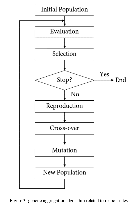
Figure 2 shows the genetic density algorithm. This network algorithm consists of seven steps with a conditional condition that we define step by step each step of this algorithm.

First Half Step of Genetic Aggregation Algorithm

1. Initial population: Different response levels are generated, each with its settings.
2. Evaluation: The created response levels should be measured using accuracy criteria. By defining the degree of tolerance, a criterion can be used to measure the contact levels of the contract.
3. Selection: The quality of each response level is determined using a cross-validation process and a smoothness measure. The best response levels are then selected to be reproduced in the next step.
4. Conditional step: After completing a complete round and in each iteration step, if the selected response levels can meet one of the two quality requirements stated in the third step or if the number of iterations is limited, Reaches its maximum, the algorithm process ends, and the final results are presented as the optimal state; Otherwise, the selected levels in the third step as the best answers go to the next step and are reproduced.

Second Half Step of Genetic Aggregation Algorithm

1. Reproduction: The best levels selected in the previous step, along with their settings, are selected as a parent (genes) to cross over with each other and jump or change (mutation).
2. Cross-over: If the parent’s selected response levels are similar, the settings for each response level are mixed; whereas if the parent’s response chosen levels are different, a linear combination of both parent response levels is generated.
3. Mutation: Optionally, changes are made to the settings of each response level; in the same way, in genetics, a child born to his parents over time has a genetic mutation.
4. New population: In this final stage, new response levels are introduced as a new city population generation. These new levels must return to the second step, their quality assessment, and continue this cycle.

Figure 2. Genetic Aggregation Algorithm Related to Response Level

The concept of cross-validation

If the number of input data for the model is too large, it increases the complexity of the model and allows calculations to be not easily performed. In such cases, cross-validation is one of how the number of input data can be optimally determined.

There are two methods for evaluating the performance of a model. In the first method, the evaluation is based on the assumptions that the model should apply. In the second method, the evaluation is based on the model’s performance in predicting new values ​​and observations. Not done. In the evaluation of the first type, it is based on the data that have been observed and used in the construction of the model, such as creating a regression model using existing laboratory data of input and output parameters based on the principle of least squares error. However, this estimated model is only possible for the observed data on which the model is based. Also, its performance cannot be measured for new data not observed at the time of modeling.

Cross-Validation Method Relies on Data

While the cross-validation method relies on data that has been obtained and observed, they have not been used at the time of modeling because the goal, in this case, is to use this existing data but to use it. It is not to measure the model’s efficiency to predict new data. Therefore, to fully evaluate the performance of a model and its optimality, we must estimate the model error based on the data left out in the cross-validation discussion. The estimation of this error is called out-of-sample error. It should be noted that the input data or design points used in estimating the output function or response level are called learning points, and the data or design points used in cross-validation to test the function or The estimated level of response are called the checking point.

Thus, cross-validation acts as a means of calculating off-sample error. The number of input data, the lower the error estimation, and the model moves towards validation. Still, if the number of this input data exceeds a certain number, the error estimation grows again. The slowness and degree of validity of the model decrease. Various methods of cross-validation include the leave-one-out method and the K-fold method.

The concept of the leave-one-out method

In this method, only one of the existing n design points is left out of the response level estimation process, and as a result, the response level based on the n-1 residual point is obtained. Then that independent design point is used to change the quality of the response surface so that the amount of response surface error for this single design point is calculated. This is done for each design point in the test environment.

Figure 3 shows an example of a one-item cross-validation method. As shown in the figure, a design point changes the response level at each stage of the validation process.

Figure 3. An Example of a Cross-Validation method of Type one

The concept of the K-fold method

In this method, the design points are divided into k layers with the same volume. This method works the same as the previous one, except several design points are left out. In the experiment design, the number k is considered to be equal to 10, and hence, the number of cross-validation calculations ends in ten iterations.

Figure 4 shows an example of a multi-layer cross-validation method performed for k = 10 layers.

Figure 4. Ax Example of a Multilayer Cross-Validation Method.

Auto refinement mechanism

Auto refinement can automatically add several design points to the model until the accuracy of the corresponding response surface reaches the user’s desired limits. This mode is used to increase the accuracy of contact surfaces using an iterative process; this means that at each iteration step, one or more design points are automatically added to estimate the contact level. Therefore, the refinement option should be enabled from the table related to the contact levels of the output parameters based on tolerance. Then the tolerance value for each output parameter should be used as the required criterion or limit for the process. Repeat defined.

This value of tolerance represents the maximum value that the output parameter can accept; thus, at each stage of the response level correction process, the maximum value of the desired parameter or output variable is calculated, and its value is compared with other maximum values ​​obtained from other correction steps. As a result, the maximum possible difference between these values ​​is detected. It is also possible to manually define your desired refinement points in the refinement points table.

Configuration Options of Refinement

The refinement section has configuration options. From the output variable combinations section, the time of application of the new modifier point can be determined. The maximum output option adds a modifier point per repetition to amplify the least accurate output. All outputs mean adding one modifier point for each output is non-convergent. The crowding distance separation percentage option is used to define the minimum allowable distance between the points of the created modifier. The number of refinement points option indicates the number of design points created during the formation of the desired response surface. The maximum number of refinement points option is also used to define the maximum number of refinement points generated during the formation of the response surface.

Figure 5 shows the settings section for correction points in the Response Levels section.

Figure 5. Settings Section for Correction Points

Figure 6 shows the iterative process of creating design points. This iterative process continues until it reaches the desired tolerance level. The horizontal axis (x-axis) represents the number of refinement points, and the vertical axis (y-axis) represents the ratio between the maximum predicted error and the tolerance of each output parameter. Convergence occurs when all output parameters are within the convergence threshold.

Figure 6. Graph of Changes in the Ratio of the Maximum Estimated Error to Tolerance in terms of Production Correction Points.

Response Surface Methodology Type: Standard Full 2nd Order Polynomial Model

The standard full 2nd order polynomials model as a response surface methodology has starting point for many design points. This model is based on a modified quadratic formulation; thus, each output parameter or variable is a quadratic function of the input parameters or variables. This method will result in satisfactory results when changes in output parameters or variables are made smoothly or gently.

In this model, write the output parameter function in terms of input variables as follows; So that the function f is a quadratic polynomial function:

Response Surface Methodology Type: Kriging Model

The kriging model is a multidimensional interpolation that combines a polynomial model similar to one of the standard response levels considered as a global model of the design space, plus a specific local deviation so that this model can intercept design points.

In this model, write the output parameter function in terms of input variables as follows; So that function f is a quadratic polynomial function (expressing the general behavior of the model), and function z is a term of deviation or turbulence (expressing the local behavior of the model):

Since the kriging model fits the contact surfaces at all design points, the goodness of fit criterion will always be appropriate. The kriging model will have better results than the standard response surface model; whenever the output parameters are stronger and nonlinear. One of the disadvantages of this model is that fluctuations can occur on the response surface.

Figure 7 shows the behavioral pattern of the function related to the kriging model. As we can see from the figure, the behavior of the estimated function consists of a general function (f) combined with a local function (z).

Figure 7. Behavioral Pattern of the Kriging Model Function.

Refinement in kriging model

In the kriging model, it is also possible to apply refinements to the design points. This model can determine the accuracy of contact surfaces and can also determine the points needed to increase accuracy. In this model, modify the design points (refinement type)  manually and automatically.

The refinement section of this model, like the previous model, has configuration options. Application of parts of the maximum number of refinement points, crowding distance separation percentage, output variable combinations, and several refinement points as in the previous model. To define the maximum percentage of relative error indicated during the process, this algorithm uses the maximum predicted relative error option.

Verification points can also be activated to detect and determine the quality of the response surface. We recommend this mode, when creating the response level using the kriging model. The operating mechanism of this type of point is that it compares the estimated values ​​of the desired output parameter and the actual values ​​observed from the same output parameter in different positions of the design space.

Verification points can also be defined automatically and manually for software. Also, if checkpoints are activated, these points will be added to the goodness of fittable.

Response Surface Methodology Type:  Non-Parametric Regression Model

The non-parametric regression model as an response surface methodology type, tends to be a general class of support vector method (RSM) techniques. The basic idea of ​​this model is that the tolerance or tolerance of the epsilon (Ԑ) forms a narrow envelope around the output response surface and extends around it. This envelope space should include all the design sample points or most of these points.

We create instability regression to estimate the regression function directly. This means that instability regression can examine the effect of one or more independent variables on a dependent variable without considering a particular function to establish the relationship between the independent and dependent variables.

Figure 8 shows the behavioral pattern of the function related to the nonparametric regression model. The behavior of the estimated function consists of a principal response surface function with a margin of tolerance on either side.

Figure 8. Behavioral Pattern of Non-Parametric Regression Model Function

In general, the features of the non-parametric regression model are:

• Suitable for non-linear responses.
• Used when the results are so-called noisy. When the number of results is enormous, this model can approximate the design points by considering a tolerance limit (Ԑ).
• It usually has a low computational speed.
• It recommends to use only when the goodness of fit criterion of the quadratic response level model does not reach the desired level.
• In some specific problems, such as lower-order polynomials, fluctuations may occur between the design points of the test environment.

Response Surface Methodology Type:  Neural Network Model

The neural network model as an response surface methodology represents a mathematical technique based on natural neural networks in the human brain. This model conects each of the input parameters to weights by arrows. They determine the active or inactive hidden functions. Also,  hidden functions are the threshold functions that are connected or disconnected to the output function based on a set of their input parameters. Finally, each time the process is repeated. This model adjusts these weight functions to minimize the error between the response levels or the same output functions with the design points or the same inputs.

Figure 9 shows the behavioral algorithm of the cellular network model. This algorithm consists of input parameters, hidden functions, and output functions.

Figure 9. Neural Network Behavior Algorithm.

In general, the features of the Neural Network model are:

• Successful for high nonlinear responses.
• The control of this algorithm is very restrictive.
• Seventy percent of the design points are learning points and thirty percent are checking points.
• Used when input parameters and the number of design points for each parameter are significant.

Response Surface Methodology Type: Sparse Grid Model

The sparse grid model is a kind of adaptive response surface; it can constantly correct itself automatically. This model is on of the response surface methodology models. This model usually requires more design points than other methods.  Users should use when the model simulation solution process is fast. This model will be usable when users use the sparse grid initialization design method. The capability of this model is that it modifies the design points only in the directions that we require. For this reason, it needs fewer design points to achieve the same quality response level. This model is also suitable for cases that involve multiple discontinuities.

Behavioral Pattern of a Distributed Network Model

Figure 10 shows the behavioral pattern of a distributed network model and how this model interpolates it hierarchically.  According to the figure below, the first cell is located at the top left and has a design point. We see the cells ‘ changes and the design points by following the cells in the horizontal and vertical directions. The peak symbol indicates the interpolation of a design point from two design points on either side of the cell. The bottom symbol indicates the division of a cell into several other cells at the location of the generated design points.

Now, if we follow the path of change of a cell and the design points in it in the horizontal direction, we see that first, we have a cell with a design point in the middle of it. This model divides that cell from the design point in the horizontal direction to the two semicircles. Also, it places the new design points of these two semicircles on its borders. This model makes Interpolation  between both cell borders, and creates new design points in the middle of these borders. As a result, it creates two design points in the middle of the two cells again.  This algorithm, divides  new cell from the two design points created into two other half-cells in the horizontal direction. The same procedure continues in the horizontal direction. According to the figure, it does all the said steps horizontally, with the same procedure in the vertical direction.

Figure 10. Spatial Network Model Behavioral Pattern.