
Dimpled Cylinder Flow Control, Paper Numerical Validation, ANSYS Fluent Training
Free
- The problem numerically simulates the water flow around a dimpled cylindrical body using ANSYS Fluent software.
- We design the 3-D model with the Design Modeler software.
- We Mesh the model with ANSYS Meshing software.
- The mesh type is Structured, and the element number equals 1966490.
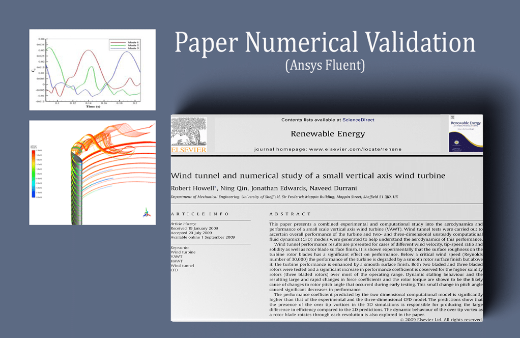
- This project is simulated and validated with a reference article.
- We aim to investigate the drag and lift forces.
To Order Your Project or benefit from a CFD consultation, contact our experts via email (info@mr-cfd.com), online support tab, or WhatsApp at +44 7443 197273.
There are some Free Products to check our service quality.
If you want the training video in another language instead of English, ask it via info@mr-cfd.com after you buy the product.
Description
Description
The present problem simulates the water flow inside a rectangular computational domain around a dimpled cylindrical body (protrusion) on its inner surface by ANSYS Fluent software.
The results of this simulation have been compared and validated with the results in the article “Control of flow past a dimpled circular cylinder“.
The fluid used in the model is water. The Reynolds number used for the fluid flow is 17980, which according to the formula for the Reynolds number, the inlet flow velocity is 0.45 m/s.
The cylindrical body is vertical and located in the direction of fluid flow within the computational domain, where the incoming water flow hits the body of its lateral surface horizontally.
As mentioned, several dimples are placed on the inner surface of this hollow cylinder; These dimples create a bulge on the inner surface and a depression on the outer surface of the cylinder.
Several patterns have been considered in the reference paper to place dimples on the cylindrical surface. In the present work, the DF (dimple full) type pattern has been used, Which means that the dimples fill the surfaces.
The geometry of the present model is drawn in three dimensions using SOLIDWORKS software. The geometry consists of a channel with a rectangular cross-section in which a hollow cylindrical body is located vertically. Dimples or bumps are also created on the inner surface of the cylinder.
These dimples are placed all over the entire body of the cylindrical body. The computational space of a rectangular cube is 6 m * 0.3 m * 0.4 m, and the cylinder has a length of 0.4 m and a diameter of 0.04 m.
The meshing has been done using ANSYS Meshing software, and the mesh type is Structured. The element number is 1966490.
Methodology
The main purpose of this work is to investigate the aerodynamic forces, including drag and lift force, on the cylinder’s outer surface and calculate drag and lift coefficients.
To calculate the drag coefficient and lift coefficient, the following equations are used, where ρ represents the fluid density, U represents the free flow velocity, and A represents the surface area that faces the fluid flow (0.4 * 0.04 = 0.016):

The simulation was performed as steady-state and transient, and the aerodynamic forces were obtained. In the transient mode, for the 60s with a time step size equal to 1s. The results showed that the changes of these aerodynamic forces in the unsteady state also become stable after a short time.
Conclusion
At the end of the solution process, we obtain the drag and lift coefficient diagram in both steady and transient modes over 60 s by taking a time step size equal to 1 s.
As the results show in the transient state, these coefficients reach an almost constant value after some time. We compare and validate these two graphs with their related graphs in the article. For this purpose, we use the DF mode in Figure 4 of the article. The following figures show the comparison and validation of the graphs.
The dimples are also modeled so that the diameter of each dimple to the diameter of the cylinder is equal to 0.1, and the depth of each dimple to the diameter of the cylinder is equal to 0.05.


At the end of the simulation, we obtain and analyze two-dimensional contours related to pressure, velocity, and velocity vectors. We draw two-dimensional contours in the X-Y section on a plane perpendicular to the body of cylindrical shapes passing through the center of this cylinder.
Reviews
You must be logged in to post a review.
Kenya Pfeffer –
Thank you for the well-presented and comprehensive training on the dimpled cylinder flow control and numerical validation using ANSYS Fluent. The detail on meshing and the thorough approach to boundary conditions provided me with an excellent insight into setting up and solving such CFD problems. The comparison with the article added rigor and validation to the training, which increased my confidence.
MR CFD Support –
We’re thrilled to hear that our training on dimpled cylinder flow control and numerical validation has been helpful to you! We pride ourselves on providing detailed simulations that align with academic research for accuracy and reliability. Thank you for the positive feedback, and we’re glad to have supported your learning journey in CFD. If you have any more questions or need further assistance, please do not hesitate to contact us.
Franz Moen –
I found this course on simulating the water flow around a dimpled cylinder very insightful. Can you provide more details on how the dimple pattern impacts the drag and lift forces compared to a smooth cylinder?
MR CFD Support –
Absolutely! Different dimple patterns modify the boundary layer behavior over the cylinder surface, which affects separation points and wake formation. The dimples increase turbulence and can potentially reduce the size of the wake, which in turn can decrease drag and affect lift characteristics. Each pattern will have a unique impact on the flow dynamics around the cylinder. Our simulation shows a detailed analysis of the DF pattern’s influence on aerodynamic forces, and the results indicate changes in drag and lift coefficients compared to a smooth cylinder due to the introduction of these dimples.
Russel Stracke –
I’m pleased with how the simulation mimics the published paper’s results. Were both steady and unsteady simulations necessary for validation, or could one have sufficed?
MR CFD Support –
Than you for your remarks. Both steady and unsteady simulations were performed to ensure comprehensive validation against the results presented in the paper. Steady simulation provides a baseline to understand the time-averaged effects, while unsteady (transient) simulation captures dynamic variations and possible fluctuations over time. Together, they offer a complete picture of aerodynamic forces’ behavior. As validation requires thoroughness, using both helps in confirming the fidelity of the simulation to the physical phenomenon being modeled.
Dr. Maximus Grant I –
After the initial transient period, how much variation do the drag and lift coefficients display over time?
MR CFD Support –
In the transient simulation, after the initial period, the drag and lift coefficients stabilize and show minimal variation over time. The coefficients reach an almost constant value, indicating that the flow has reached a quasi-steady state around the dimpled cylinder.
Mr. Rhett Kessler –
This training was incredible. Seeing the results align with the published paper was reassuring for the accuracy of the simulation process!
MR CFD Support –
Thank you so much for your positive feedback! We’re thrilled to hear that the training met your expectations and provided accurate, dependable results. Your satisfaction with the accuracy of our simulation process is our top priority.
Laura Champlin –
The training module seems very thorough. The lattice model especially helps to understand the impact of dimples on fluid dynamics around cylindrical bodies. Well done on the training content!
MR CFD Support –
Thank you for your kind words! We’re delighted that you’ve found the training module on dimpled cylinder flow control and numerical validation insightful. We strive to provide detailed and practical training content that enhances understanding of complex fluid dynamics concepts. If you have any more feedback or need further assistance, feel free to reach out.
Annie Jacobs –
The work and findings on the Dimpled Cylinder Flow Control seems impressive! Just out of curiosity, how did the presence of dimples impact the overall drag and lift coefficients compared to a smooth cylinder?
MR CFD Support –
In presence of the dimples, the flow dynamics over the cylinder surface change due to the introduction of surface disturbances, which can modify the separation points of the boundary layer. This generally affects the pressure distribution and can either increase or decrease the resulting drag and lift. Specifically, the dimpled cylinder in this simulation showed how it altered aerodynamic forces, and by comparison with the referenced paper, we could validate the behavior of the coefficients reaching a stable value, indicative of the dimples’ impact on the flow. However, for the exact numbers and analysis of drag and lift coefficient changes, you would refer to the simulation results and the comparisons made, which would detail out the quantitative impacts of the dimples compared to a smooth cylinder scenario.
Garrison Huel –
The ANSYS Meshing software you used, did it handle the complex dimpled structure without any problems and what kind of mesh quality did you achieve especially around the dimples?
MR CFD Support –
We paid special attention to meshing around the dimpled areas to ensure good accuracy in the simulation results. The structured mesh type was used, and the software managed to handle the complex geometry effectively. We achieved a high mesh quality with an enhanced focus on the regions surrounding the dimples to ensure the gradients and the flow intricacies were well-captured. Curvature and proximity refinement were employed to maintain the mesh quality and integrity, especially around the critical deep and protruding dimpled surfaces.
Lenora Bashirian –
The training and simulations were extremely educational. Seeing the fluid dynamics around the dimpled cylinder come to life with such precision is a testament to the power of computational modeling. It was fascinating to compare with the paper’s findings.
MR CFD Support –
Thank you for your kind review! We are thrilled to hear that our simulation training provided comprehensive insights into fluid dynamics and proved valuable for your understanding. It’s always rewarding to see our customers make practical connections with academic research through our CFD products.
Mrs. Providenci Stokes –
Fantastic learning content! The comparison and validation with established work gives me complete confidence in the methodology used. Your detailed exploration of dimple effects elucidates complex flow dynamics spectacularly.
MR CFD Support –
Thank you for your positive feedback! We’re thrilled to know that our efforts to provide comprehensive and trustworthy training content have met your expectations. Validation against authoritative research certainly enhances learning outcomes and understanding of fluid dynamics. If you need further assistance or have any questions, please don’t hesitate to ask.
Mr. Mavis Bosco II –
I found the simulation on a dimpled cylinder fascinating! I’m curious about how the dimples affect the flow. Do they reduce drag, and could you see any specific patterns in the flow due to the dimples during the simulation?
MR CFD Support –
Dimples on surfaces like the ones on a cylinder in fluid dynamics can affect the boundary layer and potentially reduce drag by promoting the transition to turbulence at a smaller scale, which eventually delays flow separation. We indeed observe interesting patterns in the flow due to the presence of dimples. The simulation provides insights into pressure distribution and flow behavior change, with usually a more turbulent wake behind the cylinder, which indicates energy loss and would be visible in the velocity and pressure contours around the dimpled areas. Detailed analysis in the solution phase expresses these effects explicitly.
Dr. Manley Zieme I –
I am really impressed with the comprehensive analysis and clear results from the Dimpled Cylinder Flow Control. The simulation seems thorough, and I particularly appreciate the detailed comparison with academic literature. Did the simulation take into account the effect of the dimples’ variation in size and depth or were they kept consistent throughout the model?
MR CFD Support –
Thank you for your complement! In this simulation, the dimples are consistent in size and depth throughout the model according to the specified ratio to the cylinder diameter described in the project description. The simulation adheres to the pattern detailed in the scholarly article referenced for accurate validation of the results.
Brant Keeling III –
I’m impressed by how detailed and in-depth the simulation is, especially with regards to the pattern of the dimples on the cylinder and how they affect fluid dynamics!
MR CFD Support –
Thank you so much! We’re delighted to hear that you appreciate the attention to detail in our simulation. Our team works hard to ensure accuracy and depth in our analyses, so your feedback is very rewarding for us. If you have any more questions or need further assistance, feel free to reach out!
Durward Watsica –
The training demonstrates exceptional attention to detail in parallel with the referenced paper. The application of the Dimple Full (DF) type pattern appears to be meticulously replicated to achieve validation worthy results. The clarity in explaining the setup, methodology, and resultant coefficients is noteworthy. It showcases MR CFD’s dedication to accuracy and precision in simulating complex fluid dynamics. Truly invaluable for those studying aerodynamic forces in similar contexts.
MR CFD Support –
Thank you for your insightful feedback! We’re thrilled to hear that the utility and detail of our dimpled cylinder flow control simulation met your expectations and proved useful for your studies. Your acknowledgment of the effort we put into ensuring accuracy and validation with reputable sources is very much appreciated. It motivates us to continue delivering high-quality educational content. If you have any further questions or need assistance with similar projects in the future, don’t hesitate to reach out to us.
Graciela Yost –
I’m delighted with the comprehensive training provided on Dimpled Cylinder Flow Control. The comparison with an actual research paper added confidence in the simulation approach. Will MR CFD consider creating a follow-up course detailing the impact of different dimple patterns on flow control to expand this study further?
MR CFD Support –
Thank you for sharing your positive feedback with us! We are so pleased to hear you found the training comprehensive and the comparison with research work valuable. Your interest in further expanding this study is great to hear. Currently, we do not have a follow-up course, but we will certainly take your suggestion into account as we develop new content in the future.
Mrs. Althea Thompson Sr. –
This training course seems robust and detailed. I appreciate the clarity in the description and objectives. The inclusion of real-world validation is also a selling point for me.
MR CFD Support –
Thank you for the kind words! We’re pleased to hear that you value the detail and clarity of our training, as well as the real-world application through validation. We strive to provide practical and comprehensive learning material that our customers can trust and apply. Your feedback is greatly appreciated!
Desmond Kreiger –
The training was comprehensive, clear, and the results aligned well with the reference paper! Really enhanced my understanding of aerodynamics and dimpled surface impacts.
MR CFD Support –
Thank you for your positive feedback! We’re glad to hear our training on Dimpled Cylinder Flow Control could enhance your understanding of aerodynamic influences and flow manipulation. Your appreciation is highly motivating for our team!
Roselyn Toy –
This simulation seems fascinating! I was wondering if the conclusion detail the level of agreement between the numerical simulation and the experimental results from the article? How accurately did the simulation replicate the behaviors observed in the referenced paper?
MR CFD Support –
The admin should reply to this if it mentions anywhere that they compare it to the paper cited.