k-epsilon vs k-omega vs LES: The Ultimate CFD Turbulence Guide

We’ve all been there. You spend days, maybe even weeks, setting up a complex CFD simulation. The mesh is perfect, the boundary conditions are set, and the solution converges beautifully. You generate stunning contour plots that look incredibly convincing. But when you compare the results to experimental data, they’re just… wrong. The drag is off by 20%, the heat transfer is underestimated, or the flow separation point is completely missed. More often than not, the culprit is the turbulence model.

Choosing the right turbulence model is arguably one of the most critical decisions in a CFD analysis, yet it’s a topic shrouded in complexity and academic jargon. This isn’t just a theoretical exercise; the wrong choice can invalidate your entire simulation, costing you time, computational resources, and confidence in your results.

🎯 Stop Guessing Your Turbulence Model. Download our definitive Ansys Fluent Turbulence Model Selection Flowchart — a high-res decision tree used by senior CFD engineers to pick the right model every time. 

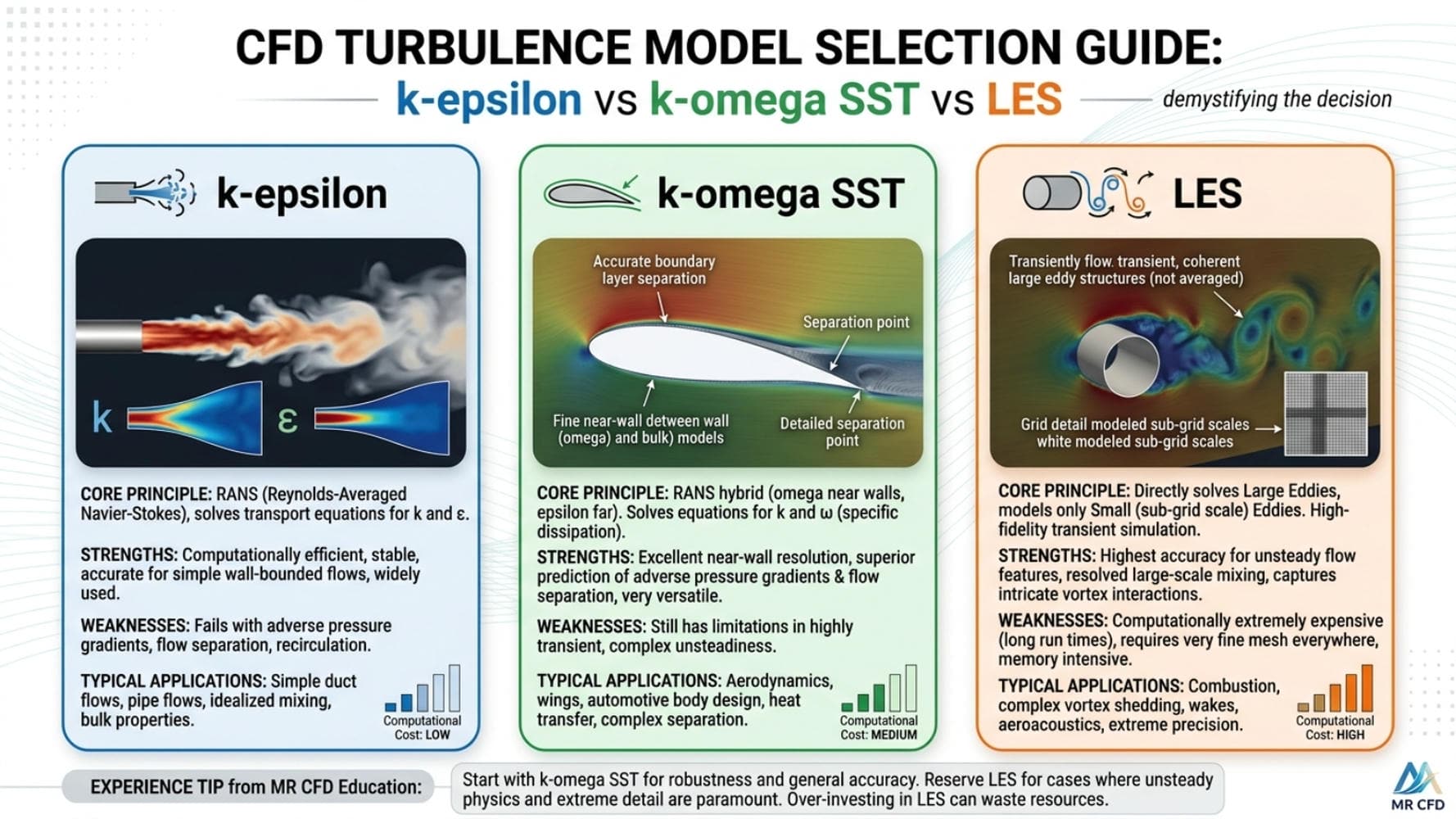
As a senior CFD educator with over a decade of experience in MR CFD, I’ve seen this issue trip up countless engineers and students. That’s why I’ve created this definitive, practical guide to the k-epsilon vs k-omega vs LES decision. Our goal is to demystify the process and provide a clear framework for selecting the appropriate model for your specific application in Ansys Fluent. We’ll move beyond simple definitions and give you the experience-based knowledge to choose between k-epsilon, k-omega, and LES with confidence.

What is Turbulence and Why is It so Difficult to Model?

Before comparing models, we must respect the enemy. Turbulence is a chaotic, three-dimensional, and unsteady fluid motion characterized by swirling structures called “eddies.” Think of the complex, churning flow of a river rapid or the smoke billowing from a chimney. These eddies exist across a vast range of sizes and time scales, from massive, energy-carrying structures down to tiny vortices where that energy is dissipated as heat.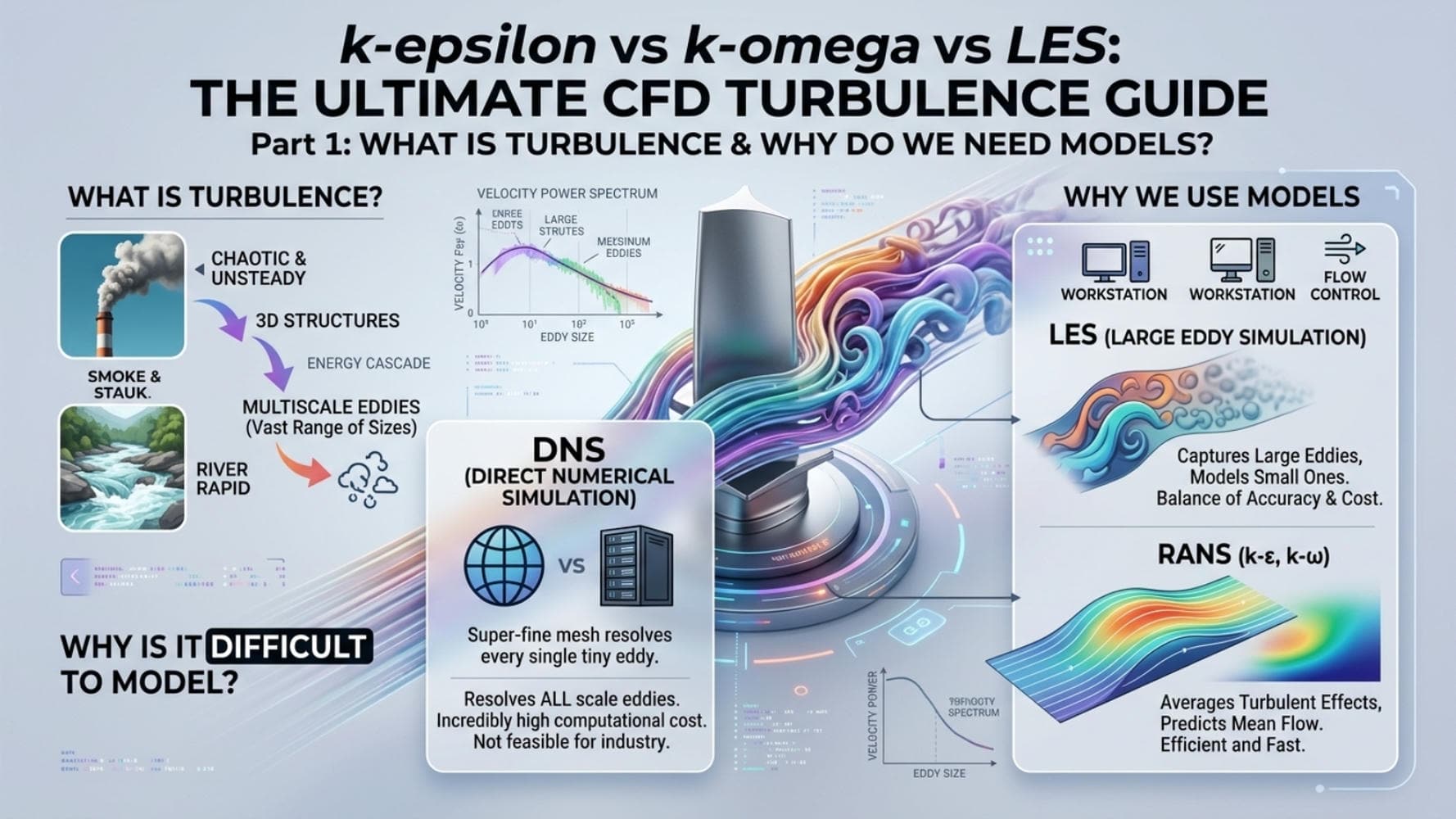

The fundamental challenge is this: the Navier-Stokes equations, which govern fluid flow, perfectly describe turbulence. However, to resolve every single eddy in a real-world engineering problem — a method called Direct Numerical Simulation (DNS) — would require a mesh so fine and time steps so small that it would take the world’s most powerful supercomputers years to solve for a simple flow over a car. It is simply not feasible for industrial applications. 

This is why we need turbulence models. They are mathematical simplifications designed to predict the effects of turbulence on the mean flow without having to compute every single eddy. Each model makes different assumptions and simplifications, which is precisely why one model can be perfect for one case and completely wrong for another.

What are the Main Categories of Turbulence Models?

Think of turbulence models as different types of tools in a toolbox, each designed for a specific job. Broadly, they fall into three main families, distinguished by the level of detail they capture and, consequently, their computational cost. Understanding these categories is the first step in making an informed decision.

k-epsilon vs k-omega vs SST vs LES: Quick-Reference Comparison Table

Before diving into the details, here is the table engineers actually need when configuring their Ansys Fluent setup. Use this as your first filter.

Model	Best Use Case	Near-Wall Treatment (Y+)	Relative CPU Cost	Flow Separation Accuracy
Standard k-ε	Fully turbulent free-shear flows, jets, plumes	Wall functions (Y+ > 30)	1x (Baseline)	Poor — misses separation
Realizable k-ε	Internal flows, swirling flows, quick industrial estimates	Wall functions (Y+ > 30)	1x	Fair — better than Standard k-ε
Standard k-ω	Wall-bounded flows, low-Re regions	Low-Y+ mesh (Y+ ≈ 1)	1x	Good near walls
SST k-ω	Aerodynamics, adverse pressure gradients, most industrial flows	Low-Y+ mesh (Y+ ≈ 1)	1x–1.5x	Excellent
DES (Hybrid)	Unsteady flows with massive separation, external aerodynamics	RANS near wall / LES in wake	5x–20x	Very Good
LES	Acoustics, combustion, highly unsteady separated flows	Very fine mesh required	50x–500x+	Excellent (if well-resolved)
DNS	Fundamental academic turbulence research	Resolves everything	1,000,000x+	Perfect (impractical industrially)

💡 Key Takeaway: For the majority of industrial Ansys Fluent setups, SST k-ω is the safest starting point. Use Realizable k-ε for free-shear flows where you need speed. Escalate to DES or LES only when unsteady vortex shedding or acoustics are the primary deliverable.

How does Reynolds-Averaged Navier-Stokes (RANS) Work?

The Reynolds-Averaged Navier-Stokes (RANS) approach is the undisputed workhorse of industrial CFD. It’s built on a simple but powerful idea: instead of resolving the chaotic, instantaneous fluctuations of turbulence, let’s just focus on the time-averaged flow properties. RANS models solve transport equations for averaged quantities and then model the effect of all turbulent eddies — from the largest to the smallest — using a concept called turbulent viscosity.

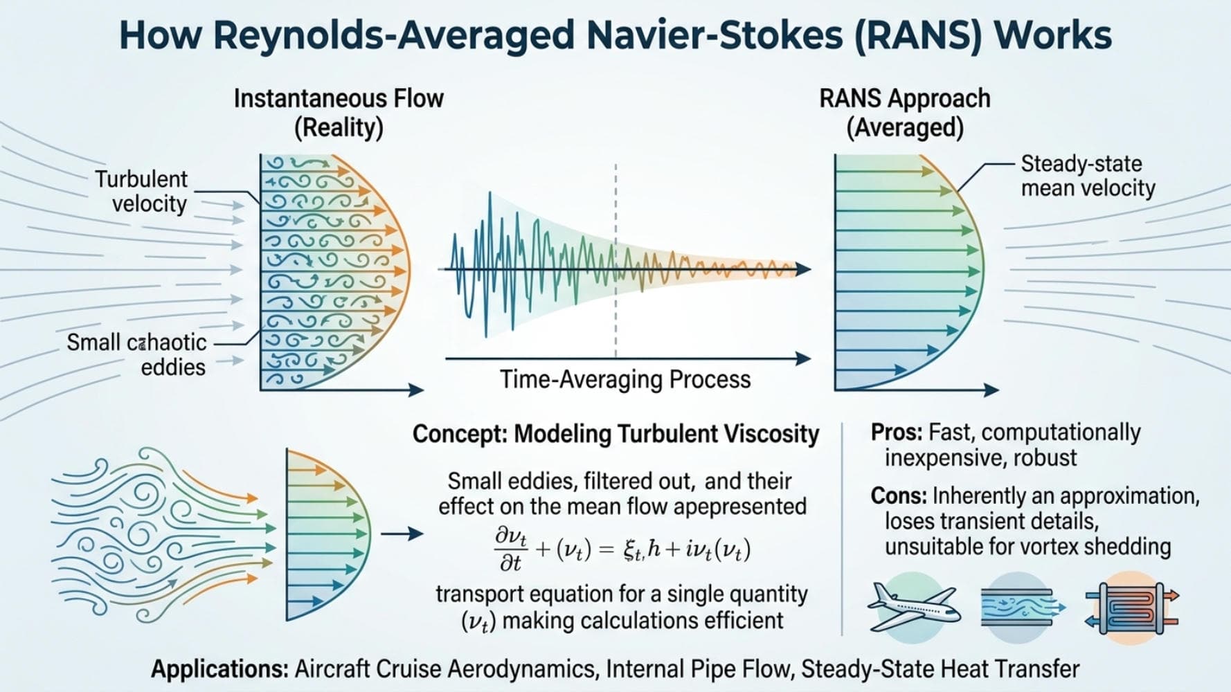
• Pros: Fast, computationally inexpensive, and robust. It provides excellent results for a wide range of steady-state applications where the large-scale turbulent structures are not the primary interest.
• Cons: It is inherently an approximation. By time-averaging, it loses all information about the transient, swirling nature of eddies, making it unsuitable for problems where flow instabilities or detailed vortex shedding are critical.

This is the go-to method for applications like aircraft cruise aerodynamics, internal pipe flow, and many steady-state heat transfer problems.

What Makes Large Eddy Simulation (LES) Different from RANS?

Large Eddy Simulation (LES) operates on a completely different philosophy. Instead of modeling everything, LES says: “Let’s resolve the big, energy-carrying eddies directly and only model the small, universal ones.” The larger eddies are highly dependent on the geometry and flow conditions, so capturing them is key to accuracy. The smaller eddies are more isotropic and behave in a more predictable way, making them easier to model with a sub-grid scale model.

• Pros: Offers significantly higher fidelity than RANS. It captures transient flow structures, making it excellent for acoustics, combustion, and flows with massive separation where RANS models fail.
• Cons: The computational cost of LES is massive — often 50–500 times higher than RANS. It requires very fine meshes and small time steps to resolve the large eddies, making it impractical for many industrial design cycles.

Where Does Detached Eddy Simulation (DES) Fit In?

So, what if you need more accuracy than RANS but can’t afford the cost of LES? This is where hybrid models like Detached Eddy Simulation (DES) come in. DES is a clever combination of the two approaches.

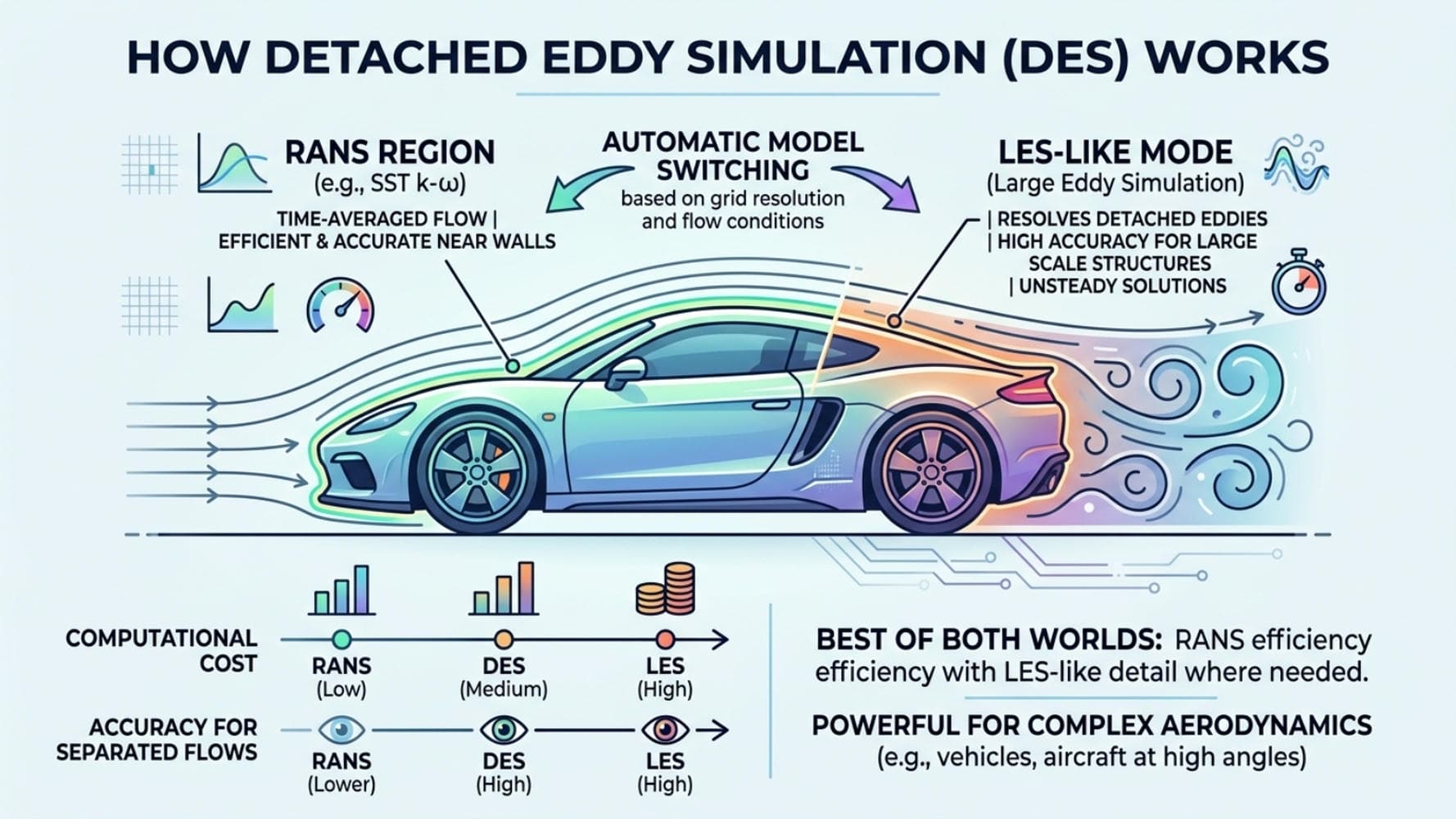
It uses a RANS model (like SST k-omega) in the thin boundary layer attached to walls, where RANS is efficient and accurate. In regions away from the wall where the flow separates and large, unsteady eddies form, the model automatically switches to an LES-like mode. This gives you the best of both worlds: the efficiency of RANS where it works best and the accuracy of LES where it’s needed most. It’s a powerful tool for complex aerodynamics — like a car or an aircraft at high angles of attack.

🚀 Need High Accuracy Without the HPC Cost? Let our consultants set up a hybrid DES/RANS model optimized for your next project. 

US Office: +1 (903) 231‑3943
UK Office: +44 7443 197273

Which RANS Model Should I Choose? A Deep Dive into k-epsilon vs k-omega

For the vast majority of CFD users, the primary question isn’t RANS vs. LES, but rather which RANS model to use. The two most prominent families are k-epsilon (k-ε) and k-omega (k-ω). This is the classic k-epsilon vs k-omega debate, and knowing the difference is crucial for getting reliable results.

When is the k-epsilon (k-ε) Model Family the Right Choice?

The k-epsilon (k-ε) model is one of the oldest and most widely used turbulence models. It’s a two-equation model that solves transport equations for two turbulent quantities: turbulent kinetic energy (k) and its dissipation rate (ε). These two variables together determine the turbulent viscosity ratio, which in turn affects how momentum is diffused throughout the flow domain.

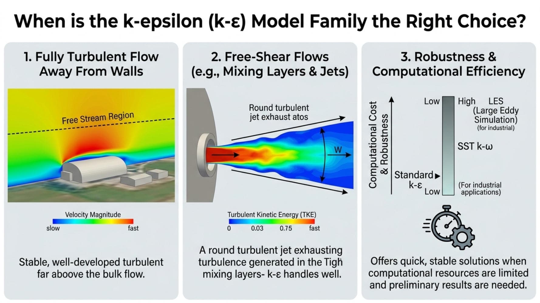
You should consider the k-ε family when:

• Your flow is fully turbulent and far from walls.
• You are simulating free-shear flows like jets, mixing layers, or plumes.
• Computational cost is a major constraint, and you need a robust, forgiving model to get a quick solution.

A common pitfall we see is using the Standard k-ε model for flows with strong adverse pressure gradients or boundary layer separation, where it is notoriously inaccurate. It relies on so-called “wall functions” to bridge the near-wall region, which can be a significant source of error if not used correctly — particularly for drag calculation errors and heat transfer underestimation.

What are the Key Differences Between Standard, RNG, and Realizable k-ε?

Not all k-ε models are created equal. In Ansys Fluent, you’ll see three options:

• Standard k-ε: The original. Robust but considered outdated for many applications due to known limitations with separated flows and strong streamline curvature.
• RNG k-ε: This variant includes improvements for rapidly strained and swirling flows, often giving better results for vortex-dominated flows or confined jets.
• Realizable k-ε: This is the most significant modern improvement within the family.

Standard vs. Realizable k-ε: Equations & Key Differences

The core distinction between Standard and Realizable k-ε lies in how turbulent viscosity (μ_t) is computed.

In the Standard k-ε model, turbulent viscosity is defined as:

μ_t = ρ · Cμ · k² / ε

where Cμ = 0.09 is a fixed empirical constant. This works well for simple flows but breaks down in regions of strong strain or rotation, where it can produce non-physical (negative) normal stresses — a violation of fundamental turbulence physics.

The Realizable k-ε model addresses this by making Cμ a variable — a function of the mean strain rate and rotation tensors:

Cμ = f(S, Ω, k, ε)

This “realizability constraint” mathematically ensures that the normal Reynolds stresses remain positive and that the Schwarz inequality for shear stresses is satisfied. In plain English: the model is prevented from producing physically impossible turbulence states.

Additionally, the Realizable k-ε uses a modified transport equation for ε that is derived from the mean-square vorticity fluctuation equation, rather than being purely empirical.

Practical result: In our experience, Realizable k-ε is the best choice within this family — particularly for flows involving jets impinging on surfaces, strong streamline curvature, and rotating flows. It consistently outperforms Standard k-ε for simulation accuracy in industrial applications.

Why is the k-omega (k-ω) Model Family Often Preferred for Wall-Bounded Flows?

The k-omega (k-ω) model is another two-equation model, but it solves for turbulent kinetic energy (k) and the specific dissipation rate (ω) — the rate at which turbulent kinetic energy is converted to thermal energy per unit volume. Its main advantage lies in how it behaves near solid walls.

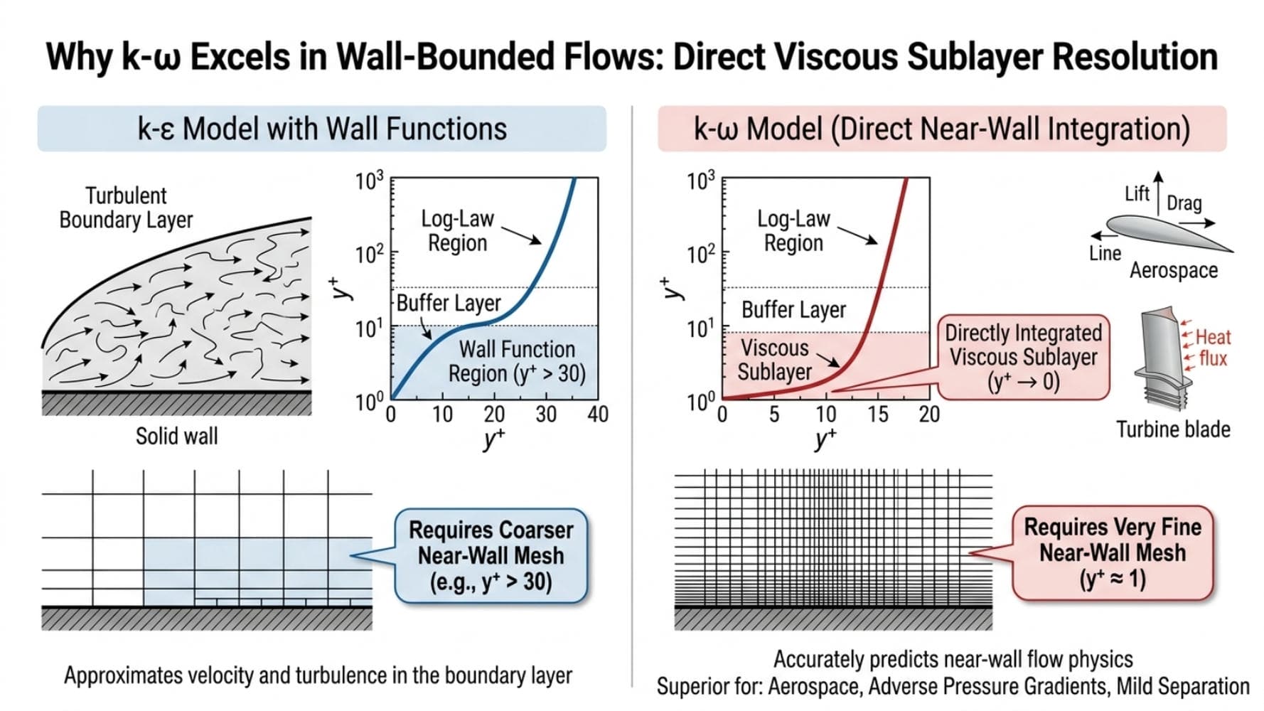
Unlike the k-ε model, the k-ω model can be integrated directly through the viscous sublayer without requiring wall functions. This makes it far more accurate for:

• Aerospace applications: Calculating lift and drag on airfoils.
• Flows with strong boundary layer effects: Heat exchangers, turbomachinery.
• Cases with adverse pressure gradients and mild separation.

This ability to resolve the flow all the way to the wall — down through the viscous sublayer and into the log-law region — is its key strength. But it comes at a price: it requires a much finer mesh in the near-wall region, with a y+ value for turbulence models targeting approximately 1.

What Makes the Shear Stress Transport (SST) k-ω Model so Popular?

The Shear Stress Transport (SST) k-ω model is arguably the most popular and versatile RANS model in use today. Developed by Florian Menter, it brilliantly combines the best features of both k-ω and k-ε.

SST k-omega explained simply:

• It uses the accurate k-ω formulation in the inner parts of the boundary layer.
• It switches to the robust k-ε formulation in the free stream, avoiding the k-ω model’s known sensitivity to freestream turbulence properties.
• It includes a critical modification to account for the transport of the principal turbulent shear stress, which significantly improves its predictions of flow separation — the single most common failure point of simpler RANS models.

Visual Proof — Why SST k-ω Beats Standard k-ε at Separation:

Consider an airfoil at a high angle of attack. The Standard k-ε model, relying on wall functions and a fixed Cμ, will typically predict attached flow well past the point where the boundary layer has physically separated. The result: drag is underestimated, lift is overestimated, and the wake region is completely wrong.

The SST k-ω model, by resolving the viscous sublayer and correctly transporting shear stress through the adverse pressure gradient region, captures the separation bubble accurately. Side-by-side contour plots of wall shear stress and velocity magnitude consistently show this: SST k-ω correctly predicts the separation onset location, while Standard k-ε misses it entirely.

This “blending” makes the SST k-ω model a highly reliable choice for a vast range of flows and our default starting point for any new CFD turbulence modeling project at MR CFD.

How Do I Decide Between RANS, LES, and DES?

Choosing the right model family requires you to step back and look at your project goals. You need to balance accuracy requirements with available resources. This is where we introduce a fundamental concept in engineering simulation.

What is the “Iron Triangle” of CFD? (Accuracy vs. Cost vs. Time)

In project management, the “Iron Triangle” states you can have a project that is Good, Fast, or Cheap — but you can only pick two. CFD has a similar trade-off:

• High Accuracy & Fast Time: Requires extremely high computational Cost (e.g., running an LES on a massive HPC cluster).
• Low Cost & Fast Time: Will likely result in lower Accuracy (e.g., a coarse-mesh RANS simulation).
• High Accuracy & Low Cost: Will take a very long Time to complete (e.g., running a fine LES on a small workstation).

Your choice of turbulence model is a direct reflection of where you want to be on this triangle. Before you even open Ansys Fluent, you must ask: “What level of accuracy is sufficient to make the required engineering decision, and what resources do I have?”

💼 Need High Accuracy Without the HPC Cost? Let our consultants set up a hybrid DES/RANS model tailored to your specific geometry and physics.

Can a Flowchart Help Me Choose the Right Turbulence Model?

Yes! To simplify this decision-making process, we’ve developed a flowchart based on our best practice guidelines. This decision tree walks you through the key questions you need to ask about your simulation.

Here’s how to use it:

1. Start with your Physics: Is your flow dominated by wall effects (aerodynamics) or is it a free-shear flow (mixing jet)? Is it largely steady, or are transient, unsteady effects like vortex shedding critical?
2. Define your Accuracy Needs: Do you need a quick, qualitative answer, or do you need validation against experimental data with high precision?
3. Assess your Resources: What is your mesh budget? Can you afford a mesh fine enough to achieve a y+ value for turbulence models of approximately 1? What is your timeline and access to computational power?

By following these questions, the flowchart will guide you to a sensible starting point — whether it’s the Realizable k-ε, SST k-ω, or a more advanced model like DES or LES.

What are the Practical Requirements for Each Model in Ansys Fluent?

Theory is great, but success in CFD comes from execution. Each turbulence model has specific meshing requirements and computational characteristics that you need to respect within the Ansys environment.

How Does Mesh Quality and y+ Affect My Model Choice?

This is the single most important practical consideration in CFD turbulence modeling. Y+ (y-plus) is a non-dimensional distance from the wall that dictates how the near-wall flow is treated. Getting it wrong is one of the fastest ways to produce a solution that looks converged but is physically incorrect.

How to Target Y+ in Ansys Fluent

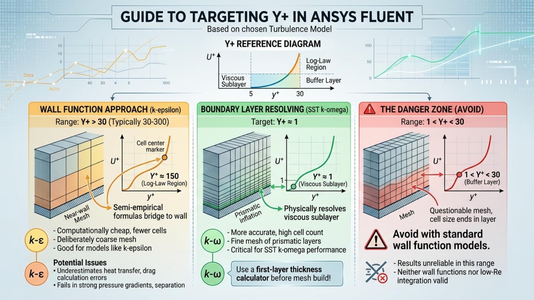
The required Y+ target depends entirely on your chosen turbulence model:

• Wall Function Approach (Y+ > 30, typically 30–300): Used with models like k-epsilon. The mesh is deliberately kept coarse near the wall, and the first cell lies in the “log-law region.” The model uses semi-empirical formulas (wall functions) to bridge the gap to the wall. It’s computationally cheap but can produce significant heat transfer underestimation and drag calculation errors if the flow involves strong pressure gradients or separation.
• Boundary Layer Resolving (Y+ ≈ 1): Required for SST k-omega to perform at its best. You must create a very fine mesh of prismatic inflation layers near the wall to physically resolve the viscous sublayer. This is more accurate but requires a significantly higher cell count. A practical rule: use a first-layer thickness calculator based on your Reynolds number and target Y+ = 1 before you build your mesh — not after.
• The Danger Zone (1 < Y+ < 30): Avoid this range with standard wall function models. The first cell falls in the buffer layer, where neither wall functions nor low-Reynolds-number integrations are valid. Results here are unreliable regardless of which RANS model you select.

🔍 Is Your Mesh Sabotaging Your SST k-omega Results? Get a free Y+ and boundary layer mesh audit from our senior CFD engineers. 

What are the Typical Computational Costs I Can Expect?

To help with planning, here is a rough estimate of the relative computational cost. A well-resolved RANS simulation is set as the baseline.

Model Category	Relative CPU Cost (Order of Magnitude)	Typical Use Case
RANS (k-ε, k-ω, SST)	1x (Baseline)	Steady-state industrial flows, aerodynamics
DES / Hybrid RANS-LES	5x–20x	Unsteady flows with massive separation
LES	50x–500x+	High-fidelity transient analysis, acoustics
DNS	1,000,000x+	Academic research on fundamental turbulence

As you can see, moving to higher-fidelity models is not a trivial decision. It represents a significant investment in computational resources that must be justified by the need for higher accuracy. For most industrial design cycles, the goal is to extract maximum accuracy from a well-configured RANS setup before escalating to DES or LES.

How Can I Master Turbulence Modeling with MR CFD?

We’ve covered a lot of ground — from the fundamental physics of turbulence to the practical k-epsilon vs k-omega vs SST vs LES comparison in Ansys Fluent. The key takeaway is that there is no single “best” turbulence model, only the most appropriate model for your specific problem, balanced against your available resources. Choosing correctly requires a solid understanding of the underlying physics, the assumptions behind each model, and the meshing discipline to execute it properly.

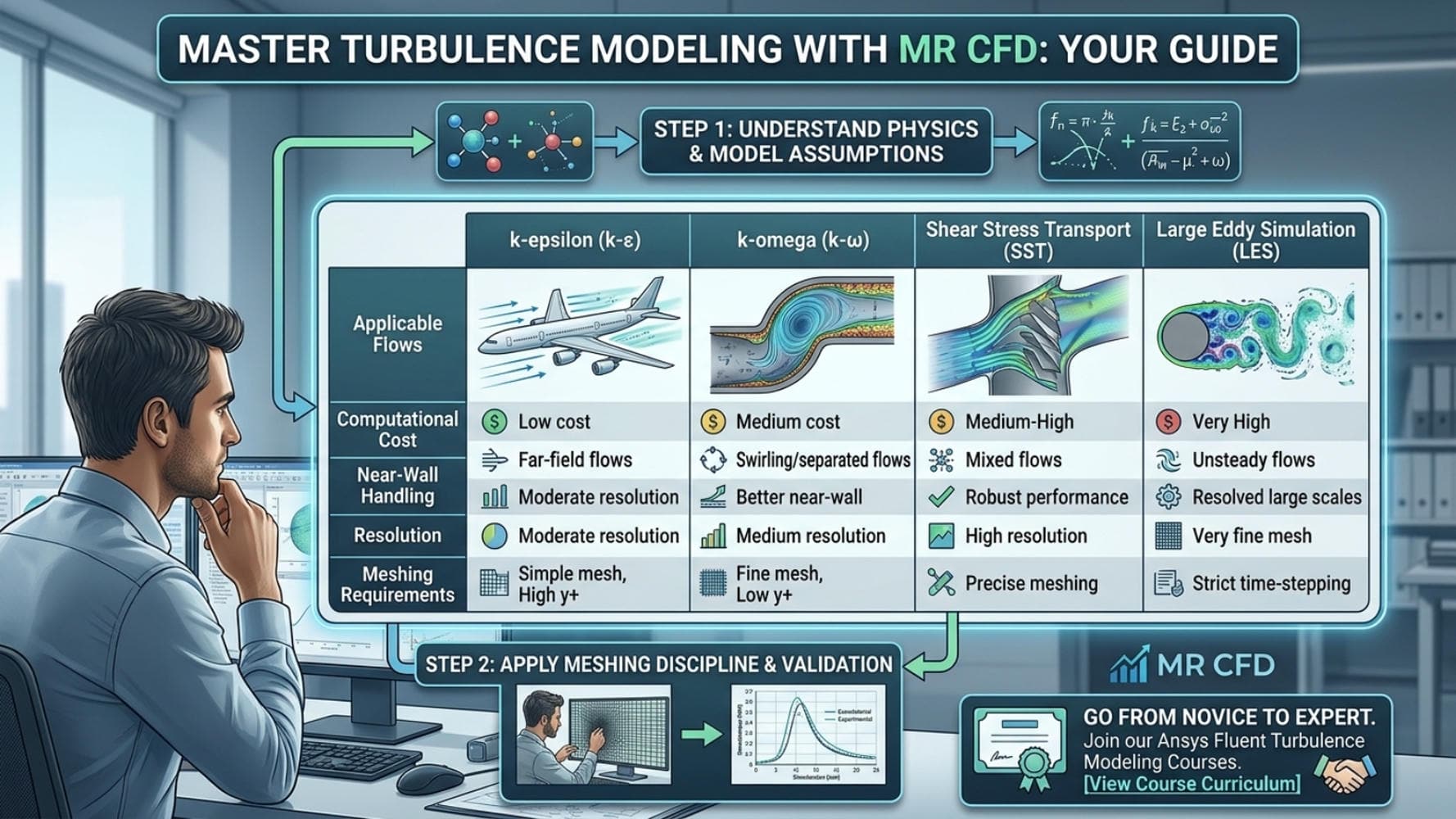
Making the right choice consistently is what separates a novice from an expert. If you’re ready to deepen your understanding and confidently apply these concepts to your own projects, MR CFD is here to help.

Our advanced CFD training courses provide hands-on experience and expert guidance, while our CFD consulting services can help you tackle your most challenging simulation problems. 🚀

Frequently Asked Questions about Turbulence Modeling

What happens if I choose the wrong turbulence model?

Choosing the wrong model can lead to significantly inaccurate results. For example, using a k-ε model for a flow that involves boundary layer separation could fail to predict the separation point correctly, leading to incorrect drag calculation errors. In the worst-case scenario, the solution might look converged and plausible but be physically wrong, leading to poor engineering decisions. The Standard k-ε is particularly prone to this in flows with adverse pressure gradients — it will often show attached flow where the boundary layer has physically separated.

Is LES always more accurate than RANS?

For flows where it is properly applied — with a sufficiently fine mesh and small time steps — LES is almost always more accurate than RANS because it resolves a much larger range of turbulent scales. However, a poorly resolved LES (where the mesh is too coarse to capture the energy-containing eddies) can be less accurate than a well-executed RANS simulation. The high computational cost of LES means that compromises are often made on the mesh, which can degrade its accuracy. Always verify that your LES mesh resolves at least 80% of the turbulent kinetic energy before trusting the results.

How do I check my y+ value in Ansys Fluent post-processing?

In Ansys Fluent, after you have a converged solution, go to the Post-Processing section. Under Plots, create a contour plot. Select “Turbulence…” as the category and then “Wall Yplus” as the variable. Display this contour on all your wall surfaces to visually inspect the values and ensure they fall within the required range for your chosen turbulence model. For SST k-ω, you want to see Y+ ≈ 1 uniformly across all walls. Any regions significantly above 5 indicate that your inflation layer is too coarse and the viscous sublayer is not being resolved — your near-wall results in those regions will be unreliable.

Can I use the SST k-omega model for any type of flow?

While the SST k-ω model is incredibly versatile and robust, it’s not a silver bullet. It is highly optimized for wall-bounded flows and aerodynamics. For flows like free jets or mixing layers far from walls, a simpler model like Realizable k-ε can sometimes perform just as well — or even slightly better — and may be more numerically stable. However, SST k-ω remains an excellent and safe default choice for the majority of industrial applications, particularly any case involving adverse pressure gradients, flow separation prediction, or boundary layer resolution.

What is the difference between turbulence intensity and turbulent viscosity ratio for setting boundary conditions?

Both are used to specify the turbulence at an inlet. Turbulence Intensity (%) is the ratio of the root-mean-square of the velocity fluctuations to the mean flow velocity — an intuitive physical parameter directly tied to the turbulent kinetic energy (k). Turbulent Viscosity Ratio is the ratio of the turbulent viscosity to the fluid’s molecular viscosity. For internal flows, it’s often easier to estimate the intensity from pipe flow correlations, while for external flows where the freestream turbulence is very low, setting a low viscosity ratio (e.g., 1–10) can be more numerically stable. Avoid setting turbulence intensity to zero — even a value of 0.1% is physically more realistic than a perfectly laminar inlet.

Does my choice of solver scheme (e.g., coupled vs. SIMPLE) affect my turbulence model’s performance?

The pressure-velocity coupling scheme primarily affects convergence speed and robustness, not the final accuracy of the turbulence model itself. However, a more robust scheme like Coupled can help stabilize a simulation struggling to converge due to complex turbulent flow features — particularly relevant for SST k-ω simulations with strong adverse pressure gradients or vortex shedding. Stabilizing convergence allows the turbulence model to reach its proper converged state, which indirectly improves result quality. For most RANS simulations, SIMPLE is adequate; switch to Coupled if you observe oscillating residuals or poor convergence behavior.

For a beginner, what is the safest and most reliable turbulence model to start with?

For a beginner tackling a wide range of industrial problems, the SST k-ω model is the safest and most reliable starting point. Its blended formulation makes it robust and effective for both near-wall and far-field flows, and it provides excellent performance for wall-bounded applications like aerodynamics and internal flows. Just remember: to get its full benefit, you must commit to creating a fine inflation mesh near the walls to achieve a y+ value for turbulence models of approximately 1. If your mesh cannot support Y+ ≈ 1 due to computational budget constraints, switch to Realizable k-ε with enhanced wall treatment as your fallback.